Python for Actuarial Students · Course 3

Lesson 8 · Part A

Production Pipelines & Model Comparison

From notebook models to production objects: scikit-learn Pipelines, penalized GLMs, persisted models, and a champion-vs-challenger test on holdout loss ratios.

Lesson 8A · OverviewBy the end of this lesson you can…

Package preprocessing and model into one Pipeline with a ColumnTransformer
Fit Poisson and Gamma GLMs in scikit-learn with exposure as a sample weight
Tune a penalized GLM’s α with grouped cross-validation
Build a gradient-boosted pipeline and recalibrate it to balance
Persist and reload models with joblib, safely and reproducibly
Run an A/B test of two pricing models on holdout loss ratios

75 min

Concepts & worked examples

75 min

Lab: champion vs challenger

Companion notebook: lesson-08a-ml-pipelines.ipynb — worked examples and self-checking exercises.

Part 1

Pipelines

One object from raw columns to prediction.

WhyWhat goes wrong between notebook and production

Failure	Example
Training/serving skew	The notebook logged mileage; the rating system didn’t
Leakage	Scaler fitted on all data before cross-validation
Unknown levels	A new vehicle style appears; the model crashes
Lost steps	“Which age bands did we use in 2025?”

A Pipeline chains transformers and a final model into one estimator. fit learns every step from training data only; predict replays them exactly. Save it, and you’ve saved the whole recipe.

Raw framestyle, age band, urban, miles

→

ColumnTransformerone-hot, log, pass-through

→

ModelPoissonRegressor

ColumnTransformerDifferent preparation for different columns

from sklearn.compose import ColumnTransformer
from sklearn.linear_model import PoissonRegressor
from sklearn.pipeline import Pipeline
from sklearn.preprocessing import FunctionTransformer, OneHotEncoder

def log_miles(miles):
    return np.log(miles / 12_000)

prep = ColumnTransformer([
    ("cat", OneHotEncoder(drop=["Sedan", "40-49"],
                          handle_unknown="ignore",
                          sparse_output=False),
     ["vehicle_style", "age_band"]),
    ("urban", "passthrough", ["urban"]),
    ("log_miles", FunctionTransformer(log_miles), ["annual_mileage"]),
], verbose_feature_names_out=False)

freq = Pipeline([("prep", prep),
                 ("glm", PoissonRegressor(alpha=0.0,
                            solver="newton-cholesky",
                            tol=1e-8))])

drop=[…] sets the base levels, like Treatment('Sedan')
handle_unknown="ignore": an unseen level scores as the base level instead of crashing
Use a named function, not a lambda: lambdas can’t be saved with joblib
"newton-cholesky" with a tight tol solves one-hot GLMs exactly

pipe[:-1].get_feature_names_out() lists the model’s columns: vehicle_style_Sports, age_band_17-20, …, urban, log_miles.

Exposurescikit-learn has no offset, and doesn’t need one

# target = claim RATE, weight = exposure
freq.fit(train, train["n_liab"] / train["exposure"],
         glm__sample_weight=train["exposure"])

freq.predict(new)                     # claims per car-year
freq.predict(new) * new["exposure"]   # expected claims

For a Poisson model with a log link, weighting the rate y/E by E gives exactly the same estimates as an offset of log E.

glm__sample_weight: the step name, two underscores, then the parameter. That’s how a Pipeline routes arguments to a step.

Coefficient	statsmodels (offset)	scikit-learn (weight)
Intercept	−3.22577	−3.22577
Sports	0.54688	0.54688
Age 17–20	0.72355	0.72355
Urban	0.31137	0.31137
log_miles	0.48786	0.48786

statsmodels for inference (standard errors, tests, summaries); scikit-learn for production (pipelines, cross-validation, persistence). Same model, same numbers.

Penalized GLMChoosing α by grouped cross-validation

PoissonRegressor(alpha=…) and GammaRegressor add an L2 (ridge) penalty α‖β‖²/2 to the deviance; the intercept is not penalized.

from sklearn.model_selection import GroupKFold
folds = GroupKFold(5, shuffle=True, random_state=0)
for tr, te in folds.split(train, groups=train["policyholder_id"]):
    for a in [0, 1e-4, 1e-3, 1e-2, 3e-2, 1e-1]:
        ...  # fit on tr, mean_poisson_deviance on te

α	CV Poisson deviance
0	0.339943
0.0001	0.339937
0.001	0.340132
0.01	0.343208
0.1	0.348671

With 64,000 car-years and 15 parameters, the data needs almost no shrinkage. At α = 0.1 every relativity is crushed toward 1 (Sports 1.03, urban 1.04): a flat rate. Penalties earn their keep with many levels and thin cells, as in Lesson 4.

Part 2

A Challenger Model

Gradient boosting in the same shape.

HistGradientBoostingscikit-learn’s own boosting

from sklearn.ensemble import HistGradientBoostingRegressor
from sklearn.preprocessing import OrdinalEncoder

GBM_FEATURES = ["vehicle_style", "driver_age", "years_licensed",
                "n_drivers", "vehicle_age", "vehicle_value",
                "annual_mileage", "urban", "coast_km"]
prep = ColumnTransformer(
    [("style", OrdinalEncoder(), ["vehicle_style"]),
     ("num", "passthrough", GBM_FEATURES[1:])],
    verbose_feature_names_out=False).set_output(transform="pandas")

def gbm(loss):
    return Pipeline([("prep", prep), ("gbm",
        HistGradientBoostingRegressor(
            loss=loss, categorical_features=["vehicle_style"],
            learning_rate=0.05, max_iter=400, max_leaf_nodes=8,
            min_samples_leaf=400, l2_regularization=1.0,
            random_state=0))])

gbm_freq, gbm_sev = gbm("poisson"), gbm("gamma")

loss="poisson" for frequency, "gamma" for severity
Native categorical support: no one-hot needed
Early stopping switches on automatically above 10,000 rows: the frequency model stopped at 59 trees
Same fit(X, rate, gbm__sample_weight=exposure) pattern as the GLM

Because both challengers are Pipelines with the same interface, the rest of the system (scoring, testing, reporting) never needs to know which one it holds.

CalibrationThe balance property, restored

@dataclass
class PurePremiumModel:
    name: str
    frequency: Pipeline
    severity: Pipeline
    freq_scale: float = 1.0
    sev_scale: float = 1.0

    def fit(self, frame):
        ...  # fit both pipelines, then:
        self.freq_scale = (frame.n_liab.sum()
            / (self.predict_frequency(frame) * frame.exposure).sum())
        self.sev_scale = (claims.inc_liab.sum()
            / (self.predict_severity(claims) * claims.n_liab).sum())

Balance factor (training)	GLM	GBM
Frequency	1.0000	0.9950
Severity	1.0000	1.0516

The boosted severity model under-predicts total losses by 5% on its own training data. A Poisson GLM with an intercept balances automatically; boosted trees don’t. Always check, and rescale before pricing.

Part 3

Persistence

Saving a model so it can be trusted later.

joblibSave, reload, verify

import joblib

model.metadata.update(
    trained_rows=66_097, trained_claims=4_041,
    sklearn_version=sklearn.__version__,     # 1.9.1
    trained_through="2024-12-31")
joblib.dump(model, "models/glm_pure_premium.joblib")   # 8.6 KB

loaded = joblib.load("models/glm_pure_premium.joblib")
np.array_equal(loaded.predict_pure_premium(hold),
               model.predict_pure_premium(hold))       # True

The GBM pair is 495 KB: 400+ trees instead of 22 coefficients.

Never load a pickle or joblib file you didn’t create. Loading runs code. Treat model files like executables: store them in controlled locations and record a checksum.

A model saved under scikit-learn 1.9 may not load under 2.0. Record library versions with the model, and pin them in the project (uv.lock).

Model governance asks: what data, which code, which version, what validation? Store the answers with the model file.

Part 4

Champion vs Challenger

An A/B test on holdout loss ratios.

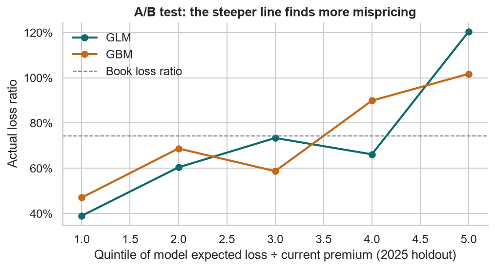
A/B testWhich model finds the mispriced risks?

for name, m in models.items():
    expected = m.predict_pure_premium(hold) * hold.exposure
    ratio = expected / hold.ep_liab     # model ÷ current premium
    q = pd.qcut(ratio.rank(method="first"), 5, labels=range(1, 6))
    lr = (hold.groupby(q).inc_liab.sum()
          / hold.groupby(q).ep_liab.sum())

Sort the 2025 holdout by what each model thinks of the current premium. Where it says “underpriced” (quintile 5), actual loss ratios should be high; where it says “overpriced”, low.

Holdout loss ratio by quintile of model expected loss over current premium: the GLM line rises from 39 percent to 120 percent, the GBM line from 47 percent to 102 percent

Scorecard2025 holdout: 18,249 vehicles, 524 claims

Metric	GLM	GBM
Frequency deviance	0.19045	0.19062
Predicted claims (actual 524)	558.7	558.9
Actual ÷ expected losses	1.014	1.043
Gini	0.275	0.235
Loss ratio, quintile 1 → 5	39.0% → 120.4%	47.0% → 101.8%

Book loss ratio 74.3%.

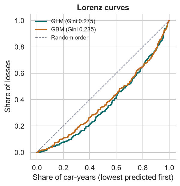
Lorenz curves of cumulative losses against cumulative car-years for the GLM and GBM

The GLM is the champion: steeper lift, higher Gini, closer A/E, and a rating table a regulator can read. The GBM stays the challenger, re-tested each year as data grows.

Actuarial Lab · 75 minChampion vs challenger

Build the GLM frequency pipeline; check its coefficients against statsmodels
Tune α over [0, 1e-4, 1e-3, 1e-2, 0.1] with GroupKFold
Build GLM and GBM severity pipelines (Gamma loss, weights = claim counts)
Wrap each pair in a PurePremiumModel with balance factors
Save both with joblib; reload; confirm identical predictions
Holdout scorecard: deviance, A/E, Gini
Loss-ratio lift by quintile; choose a champion and write two sentences why

Answer key

Best α	0.0001
GBM severity balance factor	1.052
A/E · GLM vs GBM	1.014 · 1.043
Gini · GLM vs GBM	0.275 · 0.235
GLM quintile-5 loss ratio	120.4%

RecapLesson 8A checklist

My preprocessing lives inside a Pipeline
I pass exposure as a sample weight on the claim rate
I tune penalties with grouped cross-validation
I check and restore the balance of boosted models

I save models with metadata and pinned versions
I never load model files from untrusted sources
I compare models on a holdout with lift, Gini, and A/E
I can defend the choice of champion

Up next

Lesson 8 · Part B

Capstone: A Production Pricing Engine

One command from raw policy and claim records to fitted models, rate indications, and a management report.

← Course home Next: Lesson 8B →