Capstone: A Production Pricing Engine
One command from raw policy and claim records to spatial features, fitted models, a champion-vs-challenger test, rate indications, and a management report.
Lesson 8B · OverviewBy the end of the capstone you will have…
- A Python package with a command-line entry point:
uv run pricing-engine - Validated extracts, earned exposure, and spatial features from raw records
- GLM and gradient-boosted pure-premium models in scikit-learn Pipelines
- A holdout A/B test that picks a champion on loss ratios
- A persisted production model with its metadata
- Capped rate indications in an Excel workbook and an HTML report
- Tests that prove the key calculations
Companion notebook: lesson-08b-capstone.ipynb — prototype each stage before you package it.
The briefWhat the pricing committee asked for
Capstone deliverable
A production-ready Python pricing engine that:
- ingests raw policy, vehicle, driver, coverage, and claim records
- processes exposures and spatial features
- scores policies with a regularized GLM or a gradient-boosted model, chosen by an A/B test
- exports rate indications into an automated management report
Scope: motor liability. Train on policy years 2021–2024, test on 2025, then refit the champion on all five years and rate the 2025 in-force book: 18,249 vehicles, $19.9 million of annual liability premium.
Everything you need is in Lessons 2, 3, 7, and 8A, and the Course 2 capstone showed the package pattern. This lesson is about assembling it reliably.
Architecture
Seven stages, one module each.
DesignStages and modules
pricing_engine/
├── config.toml            # every assumption
├── pyproject.toml
├── src/pricing_engine/
│   ├── extract.py       # 1 load + validate keys
│   ├── features.py      # 2 exposure, factors, spatial
│   ├── models.py        # 3 pipelines, balance, joblib
│   ├── evaluate.py      # 4 A/B test on the holdout
│   ├── indicate.py      # 5–6 refit + indications
│   ├── report.py        # 7 Excel + HTML
│   ├── cli.py           # the one command
│   └── templates/report.html.j2
├── tests/test_engine.py
└── output/ # generated, never editedEach stage takes data in and hands data out: no hidden global state. Each can be tested alone and rerun without the others.
ConfigurationAssumptions live in config.toml
[paths]
motor = "../../data/motor"
geo = "../../data/geo/nc_geo.gpkg"
output = "output"

[dates]
exposure_end = 2025-12-31
holdout_year = 2025

[age_bands]
edges = [16, 21, 25, 30, 40, 50, 65, 75, 120]
labels = ["17-20", "21-24", "25-29", "30-39",
          "40-49", "50-64", "65-74", "75+"]

[glm]
alpha = 0.0001

[champion]
model = "glm"

[indication]
target_loss_ratio = 0.68
annual_trend = 0.04
trend_years = 1.5
max_change = 0.25- Changing a trend, a cap, or the champion is a config change, reviewed like any other, with no code edit
- The first age edge is 16, not 17: an unrounded age of 16.998 would otherwise fall outside every band and silently become
NaN - The champion is a decision made from the A/B test, then recorded
Read it with the standard library: tomllib.load(open(path, "rb")). TOML dates arrive as datetime.date.
Building the Stages
Raw records to scored policies.
Stages 1–2Extract, exposure, and spatial features
def earned_exposure(start, expiry, cancel, end):
    stop = pd.concat([expiry, cancel], axis=1).min(axis=1) \
             .clip(upper=end)
    return ((stop - start).dt.days + 1).clip(lower=0) / 365.25

def spatial_features(policies, geo_path):
    pts = gpd.GeoDataFrame(policies[["policy_id"]], crs="EPSG:4326",
            geometry=gpd.points_from_xy(policies.longitude,
                                        policies.latitude)
          ).to_crs("EPSG:32119")                 # meters
    counties = gpd.read_file(geo_path, layer="counties")
    places = gpd.read_file(geo_path, layer="places")
    coast = gpd.read_file(geo_path, layer="coastline")
    out = gpd.sjoin_nearest(pts, counties, how="left")
    out["urban"] = out.within(places.union_all())
    out["coast_km"] = out.distance(coast.union_all()) / 1000
return pd.DataFrame(out.drop(columns="geometry"))extract.load_tablesrefuses to continue on a duplicate key or an orphan foreign key (Course 2)- Exposure stops at the earliest of expiry, cancellation, and the evaluation date
- Driver features: youngest driver’s age and years licensed at inception
- Spatial: county, urban (inside an incorporated place), distance to the coast
Result: 84,346 vehicle-terms, 72,781 car-years, 4,565 liability claims, one row each, saved as output/model_frame.parquet.
Stages 3–4Two candidates, one holdout
train = frame[frame.policy_year < holdout_year]
hold = frame[frame.policy_year == holdout_year]

candidates = models.build_models(cfg["glm"], cfg["gbm"])
for m in candidates.values():
    m.fit(train)                    # freq + sev + balance
metrics = evaluate.holdout_metrics(candidates, hold)
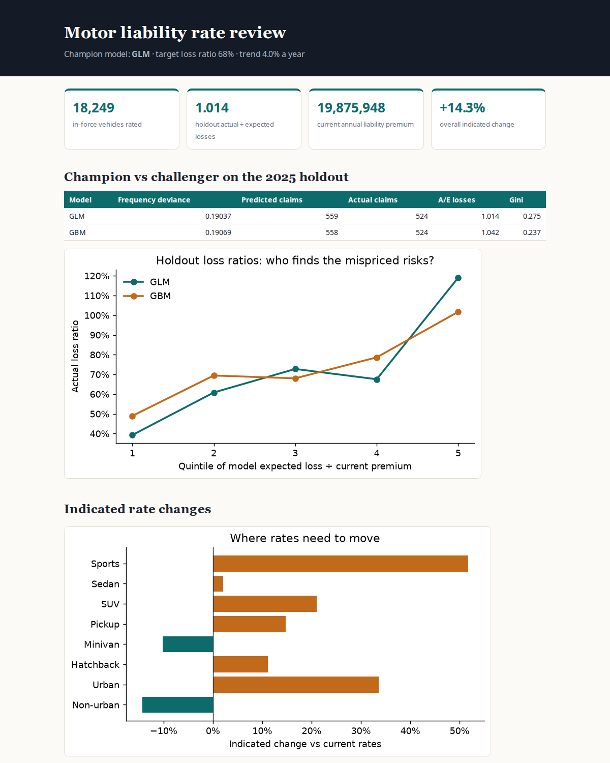
lift = evaluate.loss_ratio_lift(candidates, hold)| 2025 holdout | GLM | GBM |
|---|---|---|
| A/E losses | 1.014 | 1.042 |
| Gini | 0.275 | 0.237 |
| Loss ratio, quintile 1 → 5 | 39.3% → 119.1% | 49.0% → 101.7% |
Same verdict as Lesson 8A: the GLM is champion. Record it in config.toml (model = "glm").
Numbers differ slightly from 8A’s because the engine rebuilds its features from raw records: ages aren’t rounded, for instance. A pipeline that reproduces its own inputs is the point.
Stages 5–6Production refit and rate indications
champion = build_models(...)[name].fit(frame)   # all 5 years
champion.metadata.update(trained_through="2025-12-31",
                         holdout=metrics.loc[name].to_dict())
champion.save(out / "models" / "glm_pure_premium.joblib")

trend = (1 + annual_trend) ** trend_years        # 1.04 ** 1.5
indicated = champion.predict_pure_premium(book) \
            * trend / target_loss_ratio
change = indicated.sum() / book.liab_premium.sum() - 1
proposed = change.clip(-max_change, max_change)
$$\text{Indicated premium} = \frac{\text{Pure premium} \times (1+\text{trend})^{t}}{\text{Target loss ratio}}$$
| Segment | Vehicles | Indicated | Proposed |
|---|---|---|---|
| All | 18,249 | +14.3% | — |
| Urban | 10,902 | +33.6% | +25.0% |
| Non-urban | 7,347 | −14.3% | −14.3% |
| Sports | 1,238 | +51.7% | +25.0% |
| SUV | 4,972 | +21.0% | +21.0% |
| Sedan | 5,583 | +2.1% | +2.1% |
| Minivan | 1,272 | −10.2% | −10.2% |
| Age 17–20 | 666 | +45.3% | +25.0% |
| Age 65–74 | 1,258 | +0.0% | +0.0% |
| Age 75+ | 876 | +33.0% | +25.0% |
Stage 7The management report
rate_review.xlsx: Summary cards, Model comparison, Loss ratio lift, Indications, Rating factorsrate_review.html: one self-contained page (charts embedded as base64 PNG), rendered from a Jinja2 template- Both regenerated by every run; nobody edits them by hand
The headline for the committee: overall +14.3%, driven by urban risks the current plan doesn’t rate. The ±25% cap leaves the urban, Sports, and youngest-driver indications partly unaddressed, a decision for the committee, not the code.
Run It, Test It
Trustworthy because it’s checked.
One commandFrom raw data to report in about 20 seconds
$ uv run pricing-engine --config config.toml
INFO    pricing_engine.extract: loaded policies          78,062 rows
INFO    pricing_engine.extract: loaded claims            11,562 rows
INFO    pricing_engine.extract: all primary and foreign keys valid
INFO    pricing_engine.features: frame: 84,346 vehicle-terms, 72,781 car-years, 4,565 liability claims
INFO    pricing_engine.models: glm fitted: balance factors frequency 1.0000, severity 1.0000
INFO    pricing_engine.models: gbm fitted: balance factors frequency 0.9950, severity 1.0516
INFO    pricing_engine.evaluate: glm: A/E 1.014, Gini 0.275
INFO    pricing_engine.evaluate: gbm: A/E 1.042, Gini 0.237
INFO    pricing_engine.models: saved glm model to glm_pure_premium.joblib
INFO    pricing_engine: overall indicated change +14.3%
INFO    pricing_engine.report: wrote rate_review.xlsx
INFO    pricing_engine.report: wrote rate_review.html
The log is an audit trail: row counts, key checks, balance factors, and the A/B result, every run. Add -v for debug detail.
TestsProve the calculations, not just the plumbing
def synthetic_book(n=20_000, seed=0):
    """Known truth: urban claims 30% more often;
    Sports claims cost 40% more."""
    ...

def test_glm_recovers_known_relativities_and_balances():
    book = synthetic_book()
    glm = build_models(GLM, GBM)["glm"].fit(book)
    assert (glm.predict_frequency(book) * book.exposure).sum() \
        == pytest.approx(book.n_liab.sum())
    ...
    assert urban == pytest.approx(1.3, abs=0.08)
assert sports == pytest.approx(1.4, abs=0.1)| Test | Proves |
|---|---|
| exposure stops at cancellation and evaluation date | Earned exposure is right |
| GLM recovers known relativities and balances | The model can find a planted truth |
| GBM is rebalanced to training totals | Calibration works |
| proposed changes are capped | The cap is enforced |
| downtown Raleigh is urban, in Wake County | The spatial join is right |
$ uv run pytest -q
.....                                  [100%]
5 passed
Capstone · at your own paceBuild steps and checkpoints
- Prototype each stage in the companion notebook
uv init --package pricing-engine; add dependencies; create the modules- Extract + features: match 84,346 rows and 4,565 claims
- Models: GLM and GBM
PurePremiumModels with balance factors - Evaluate: holdout A/E, Gini, and loss-ratio lift for both
- Refit the champion on all years; save it with metadata
- Indications by urban, style, and age band, capped at ±25%
- Excel + HTML report; the CLI; at least five tests
Checkpoints
| Car-years · liability claims | 72,781 · 4,565 |
| Holdout A/E: GLM · GBM | 1.014 · 1.042 |
| Holdout Gini: GLM · GBM | 0.275 · 0.237 |
| Current premium (in-force) | 19,875,948 |
| Overall indicated change | +14.3% |
| Urban indicated change | +33.6% |
Going furtherExtensions
- Interactions: add young × sports to the GLM (Lesson 7) and re-run the A/B test
- Tweedie challenger:
TweedieRegressor(power=1.6)orHistGradientBoostingRegressor(loss="tweedie")as a third model - Territories: county relativities with a penalized GLM, so thin counties shrink toward the state average
- Off-balance: after capping, rebalance so the total change equals the committee’s approved figure
- Monitoring: a
scorecommand that loads the saved model and reports A/E on new data each quarter - Other coverages: collision and comprehensive, with coverage-specific exposure (Course 2, Lesson 4)
- Explanations: a SHAP waterfall per policy for the GBM challenger
- Model card: a Markdown page with data, method, validation, and limitations, generated with the report
A capstone reviewer will ask: can I rerun it, does it reproduce your numbers, and do the tests fail when a calculation breaks? Build for those three questions.
RecapCourse 3 checklist
- OLS and its failure modes; log models and robust SEs
- Poisson and negative binomial frequency with exposure offsets
- Gamma severity, frequency × severity, and Tweedie pure premium
- Validation, cross-validation, Lasso, Ridge, and ElasticNet
- K-means risk groups and how to choose and explain k
- Surrogate trees that turn clusters into rules and tiers
- Boosting with actuarial losses, and SHAP explanations
- Pipelines, persistence, A/B tests, and a working pricing engine
Production Actuarial Systems, Software Engineering & Enterprise Deployment
From working code to robust software: design patterns, automated testing, CI/CD, dashboards, and actuarial simulation engines.