Python for Actuarial Students · Course 3

Lesson 7

Modern Non-Linear Modeling: Gradient Boosting & Trees

Models that find curves and interactions on their own, how to make them speak actuarial (Poisson deviance, exposure), and how SHAP makes them explain themselves.

Lesson 7 · OverviewBy the end of this lesson you can…

Name the limits of GLMs: hand-built shapes and interactions
Explain how CART regression trees split, and why one tree isn’t enough
Contrast random forests (bagging) with gradient boosting
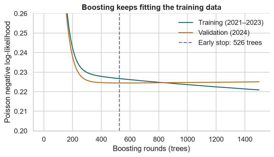
Train XGBoost with a Poisson objective and an exposure offset, with early stopping
Compare models fairly with grouped cross-validation and a holdout year
Explain predictions globally and per policy with SHAP values

75 min

Concepts & worked examples

75 min

Lab: XGBoost frequency + SHAP

Companion notebook: lesson-07-gradient-boosting.ipynb — worked examples and self-checking exercises.

Part 1

Where GLMs Need Help

Everything non-linear is your job.

LimitationsA GLM only knows what you tell it

Shapes: the U in driver age needed bands (Lesson 2); mileage needed a log
Interactions: every combination effect must be written as a term
Search: with 20 features there are 190 pairwise interactions to consider

train["young_sports"] = ((train["driver_age"] < 25)
                         & (train["vehicle_style"] == "Sports"))
glm_i = smf.glm("n_liab ~ " + rhs + " + young_sports", ...).fit()
# young_sports IRR 1.407 (1.148–1.724)
# Sports IRR 1.728 → 1.526;  AIC 30,212.5 → 30,203.8

Lesson 2’s Sports relativity of 1.73 was inflated by an interaction we didn’t model. Once we know to add it, the GLM finds it: young driver × sports car = 1.41 (truth 1.60), and Sports falls toward its truth of 1.40.

But we knew because we built the data. In real work, which interaction should you add? Tree ensembles search for them automatically.

Part 2

Trees and Ensembles

CART, random forests, gradient boosting.

CARTA regression tree for claim frequency

from sklearn.tree import DecisionTreeRegressor
cart = DecisionTreeRegressor(criterion="poisson",
                             max_depth=3, min_samples_leaf=500)
# target = claims per car-year, weighted by exposure
cart.fit(X_tr, y_tr / e_tr, sample_weight=e_tr)

|--- driver_age <= 25.2
|   |--- style_Sports <= 0.5
|   |   |--- annual_mileage <= 13650 ...
|   |--- style_Sports >  0.5 ...
|--- driver_age >  25.2
|   |--- annual_mileage <= 12250 ...
|   |--- annual_mileage >  12250
|   |   |--- urban <= 0.5 ...

Splits greedily to reduce Poisson deviance, the right loss for counts
Interactions are built in: the Sports split only happens inside the young-driver branch
Weighting the rate by exposure is equivalent to a Poisson offset

One tree is a step function with 8 values. It’s unstable (a small data change can flip the first split) and coarse. Holdout Gini 0.162 vs the GLM’s 0.220.

EnsemblesMany trees: bagging vs boosting

Random forest (bagging)

Hundreds of deep, independent trees, each on a bootstrap sample and a random subset of features
Average their predictions → variance falls
Hard to overfit by adding trees; few settings to tune

RandomForestRegressor(n_estimators=300,
    criterion="poisson", min_samples_leaf=200,
    max_features=0.5)

Gradient boosting

Hundreds of shallow, sequential trees; each fits what the previous ones got wrong (the gradient of the loss)
Add each tree’s prediction, shrunk by a learning rate η → bias falls
Can overfit: stop early on a validation set

$$F_m(\mathbf{x}) = F_{m-1}(\mathbf{x}) + \eta\, h_m(\mathbf{x})$$

Implementations: XGBoost, LightGBM, CatBoost, scikit-learn’s HistGradientBoostingRegressor.

Part 3

XGBoost for Claim Frequency

A Poisson objective, an exposure offset, early stopping.

Actuarial lossesTeaching XGBoost about exposure

import xgboost as xgb

val = train["policy_year"] == 2024     # validation year
dtr = xgb.DMatrix(X[~val], label=y[~val],
                  base_margin=np.log(expo[~val]))   # offset!
dva = xgb.DMatrix(X[val], label=y[val],
                  base_margin=np.log(expo[val]))

params = {"objective": "count:poisson",   # log link
          "eta": 0.03, "max_depth": 3,
          "min_child_weight": 50,          # credibility floor
          "subsample": 0.8, "colsample_bytree": 0.8,
          "eval_metric": "poisson-nloglik"}
bst = xgb.train(params, dtr, num_boost_round=3000,
                evals=[(dtr, "train"), (dva, "valid")],
                early_stopping_rounds=100)
bst.best_iteration + 1                   # 526 trees

count:poisson: Poisson deviance, log link, as in the GLM
base_margin = log(exposure) is the offset
For severity: reg:gamma; for pure premium: reg:tweedie with tweedie_variance_power
LightGBM: objective="poisson", init_score= log exposure

Training loss keeps falling with boosting rounds while validation loss flattens; early stopping at 526 trees

Fair comparisonFive-fold cross-validation, grouped by policyholder

Model (policy years 2021–24)	Mean Poisson deviance	vs GLM
GLM on raw features (linear age, raw miles)	0.34327	+0.00332
Random forest	0.34199	+0.00205
XGBoost (Poisson)	0.34082	+0.00087
GLM, engineered (age bands, log miles)	0.33994	—
GLM, engineered + young × sports	0.33989	−0.00005

XGBoost beats the raw-feature GLM in all 5 folds, and loses to the engineered GLM in all 5.

This book’s true risk model is a multiplicative GLM, and a GLM with the right shapes is hard to beat. Boosting’s value was finding those shapes without being told. On real portfolios, with messier structure, boosting often wins outright.

The 2025 holdout (524 claims) is too small to separate the top models: deviance 0.19036 (XGBoost) vs 0.19047 (GLM); Gini 0.223 vs 0.220. Only the raw-feature GLM (0.19226) is clearly worse.

Part 4

SHAP

Opening the black box, one prediction at a time.

TheoryShapley values: fair credit for a prediction

$$f(\mathbf{x}) = \phi_0 + \sum_{j=1}^{p}\phi_j(\mathbf{x})$$

φ₀: the average prediction (base value)
φ_j: feature j’s contribution for this policy, averaged over every order in which features could be added (Shapley, 1953)
Contributions always add up exactly to the prediction

# XGBoost computes exact TreeSHAP itself.
# base_margin = 0 → explain the log ANNUAL claim rate
d = xgb.DMatrix(X_hold, base_margin=np.zeros(len(X_hold)))
phi = bst.predict(d, pred_contribs=True)   # last col = φ0
phi[0, -1]            # −2.756 → e^−2.756 = 0.0636 per year

With a log link, SHAP values live on the log scale, so e^φ_j is a multiplicative relativity for this one policy. It’s a per-policy rating factor.

The shap package draws the plots: wrap XGBoost’s values in shap.Explanation(values, base_values, data, feature_names), then call shap.plots.beeswarm or shap.plots.waterfall.

GlobalWhat drives the model, and which way

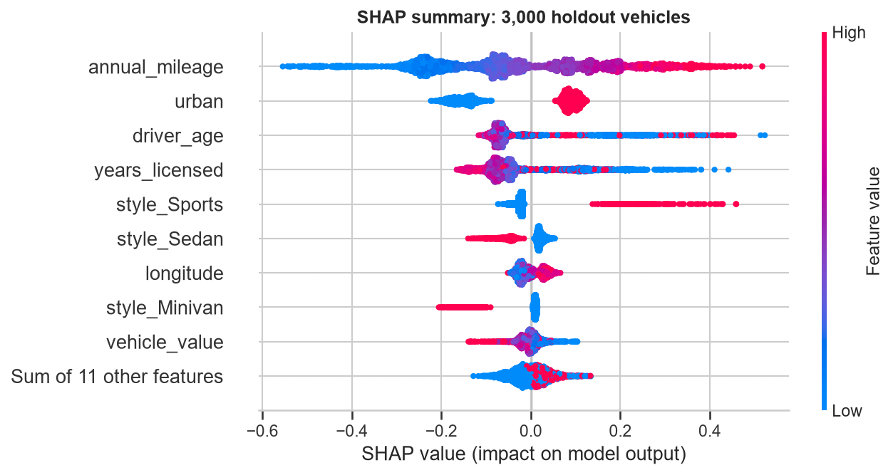
SHAP beeswarm plot: annual mileage, urban, driver age, years licensed and Sports have the largest contributions

Feature	Mean \|φ\|
annual_mileage	0.171
urban	0.116
driver_age	0.090
years_licensed	0.087
style_Sports	0.039

One dot per vehicle; color = feature value. Gender and channel: ≤ 0.004.

Age and years licensed carry the same information, so the model splits the credit between them.

ShapesThe model found the curves on its own

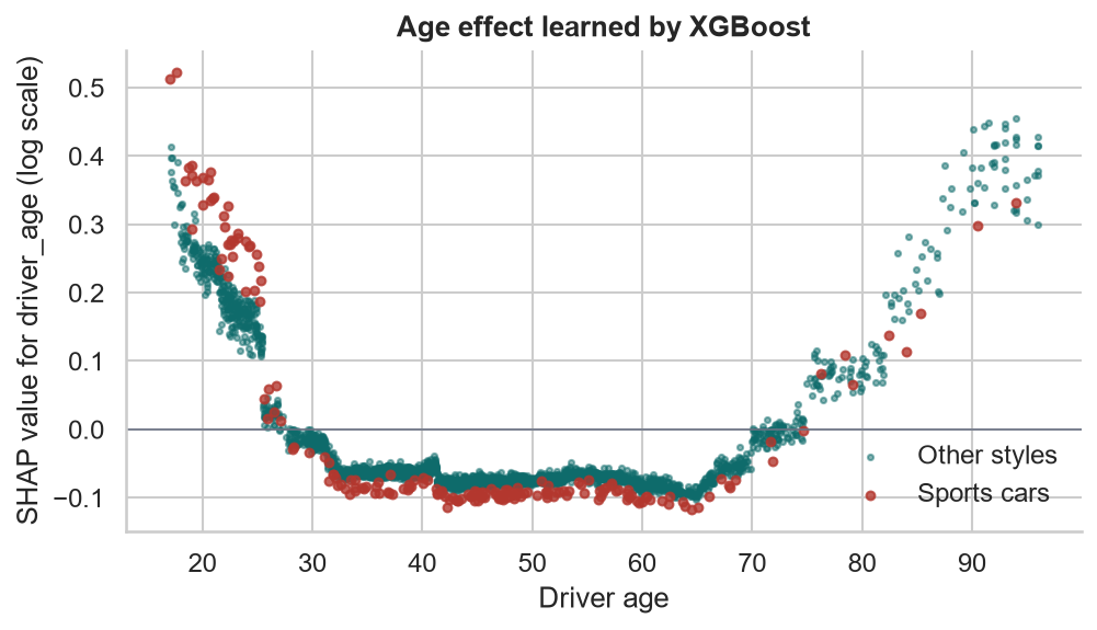
SHAP value for driver age: high for drivers under 25, flat through middle age, rising after 70; sports cars highest among young drivers

The U in age, with no bands. Young sports-car drivers (red) sit highest.

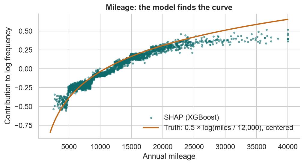
SHAP value for mileage tracks the true square-root-of-mileage curve up to about 25,000 miles

Mileage follows the true 0.5 × log(miles) curve, flattening where data runs out above 25,000.

LocalWhy is this driver’s rate high?

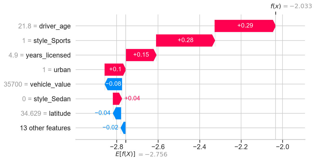
SHAP waterfall for a 21.8-year-old urban sports-car driver: driver age +0.29, Sports +0.28, years licensed +0.15, urban +0.10, vehicle value -0.08

A 21.8-year-old, urban, sports car, 12,200 miles:

Base φ₀	−2.756	0.0636
driver_age	+0.293	× 1.34
style_Sports	+0.282	× 1.33
years_licensed	+0.147	× 1.16
urban	+0.101	× 1.11
vehicle_value	−0.082	× 0.92
Prediction	−2.033	0.131 per year

Smaller contributions from other features make up the rest.

InteractionsSHAP interaction values: a lead, not a verdict

inter = bst.predict(d, pred_interactions=True)
# inter[i, j, k]: policy i's joint effect of features j and k

Pair (mean \|interaction\|)	Value	In the truth?
annual_mileage × urban	0.028	No
driver_age × style_Sports	0.011	Yes
annual_mileage × style_Sedan	0.010	No

For young sports-car drivers, the age and license × Sports interactions add +0.221: × 1.25 (truth × 1.60).

The top-ranked “interaction” isn’t real: the model is approximating a smooth multiplicative surface with step functions, and that leaves interaction-shaped residue.

The professional workflow: use boosting + SHAP to find candidate shapes and interactions, then test them in the GLM with likelihood-ratio tests and holdout data. The GLM stays the filed, explainable rating plan.

Actuarial Lab · 75 minXGBoost claim frequency with SHAP

Build a numeric feature matrix: one-hot style and channel, 0/1 urban and male
Train XGBoost (count:poisson, base_margin = log exposure) on 2021–23, early-stopping on 2024
Refit on 2021–24 with the chosen number of trees
Five-fold GroupKFold: raw GLM, engineered GLM, XGBoost
SHAP: beeswarm, age and mileage dependence, one waterfall
Find the strongest interactions; test young × sports in the GLM with an LR test

Answer key

Early-stopped trees	526
CV deviance: raw GLM · XGB · GLM	0.3433 · 0.3408 · 0.3399
SHAP base rate	0.0636
Top feature by mean \|φ\|	annual_mileage
young_sports IRR in the GLM	1.407
AIC with the interaction	30,203.8

RecapLesson 7 checklist

I know what a GLM can’t find on its own
I can explain CART, bagging, and boosting
I train XGBoost with a Poisson objective and a log-exposure offset
I stop boosting early on a validation year

I compare models with grouped CV, not a single lucky split
I read SHAP values as per-policy log relativities
I treat interaction rankings as leads to test, not facts
I use boosting to improve the GLM, not only to replace it

Up next

Lesson 8 · Part A

Production Pipelines & Model Comparison

scikit-learn Pipelines, penalized GLMs, persisting models with joblib, and an A/B test on holdout loss ratios.

← Course home Next: Lesson 8A →