Rule Extraction & Interpretability of Unsupervised Models
A centroid in ten-dimensional space won’t fit in an underwriting manual. A decision tree that imitates the clusters will.
Lesson 6 · OverviewBy the end of this lesson you can…
- Explain why cluster assignments need translating into rules
- Fit a surrogate
DecisionTreeClassifierto predict cluster labels - Measure a surrogate’s fidelity on members it hasn’t seen
- Control complexity with
max_depth, leaf sizes, and pruning - Export readable rules with
export_textandplot_tree - Map members into risk tiers and test them on next year’s cost
Companion notebook: lesson-06-rule-extraction.ipynb — worked examples and self-checking exercises.
The Post-Clustering Challenge
From latent centroids to business rules.
The problem“Nearest centroid in standardized log space”
Lesson 5’s K-means assigns a member by:
- log1p-transforming ten features
- subtracting 2024 means and dividing by 2024 standard deviations
- computing Euclidean distance to three centroids
- picking the smallest
Accurate, but no underwriter, regulator, or care manager can apply it or check it by hand.
Surrogate modeling: train an interpretable model to predict the complex model’s output. Here the target is the cluster label, not cost. The surrogate’s job is to imitate, and its score is fidelity: how often it agrees with the clusters.
Surrogate Decision Trees
Imitate the clusters with a few questions.
CARTHow a classification tree grows
- Consider every feature and every threshold: “active_months ≤ 8.5?”
- Pick the split that makes the two children purest (lowest Gini impurity)
- Repeat inside each child
- Stop at a depth or leaf-size limit; each leaf predicts its majority class
$$\text{Gini}(t) = 1 - \sum_c p_c(t)^2$$
0 for a pure leaf; 0.667 for three equally mixed classes.
from sklearn.model_selection import train_test_split
from sklearn.tree import DecisionTreeClassifier

feats = prof                      # raw units: counts, $, months
y = cluster                       # names from Lesson 5
X_tr, X_te, y_tr, y_te = train_test_split(
    feats, y, test_size=0.3, random_state=0, stratify=y)

tree = DecisionTreeClassifier(max_depth=2, random_state=0)
tree.fit(X_tr, y_tr)
tree.score(X_te, y_te)            # fidelity 0.9625
Fit on raw units, not the scaled logs: the rules come out as “9 or more active months” and “$25,438 allowed”, not “z > 0.41”.
ComplexityHow deep should the tree be?
| max_depth | Leaves | Training fidelity | Test fidelity |
|---|---|---|---|
| 1 | 2 | 0.902 | 0.906 |
| 2 | 4 | 0.963 | 0.963 |
| 3 | 8 | 0.970 | 0.966 |
| 4 | 15 | 0.975 | 0.967 |
| 6 | 42 | 0.985 | 0.969 |
| 10 | 102 | 0.996 | 0.971 |
| unlimited | 138 | 1.000 | 0.970 |
max_depth: the number of questions on any pathmin_samples_split: don’t split a node smaller than thismin_samples_leaf: every leaf must hold at least this many members, which is a credibility floor
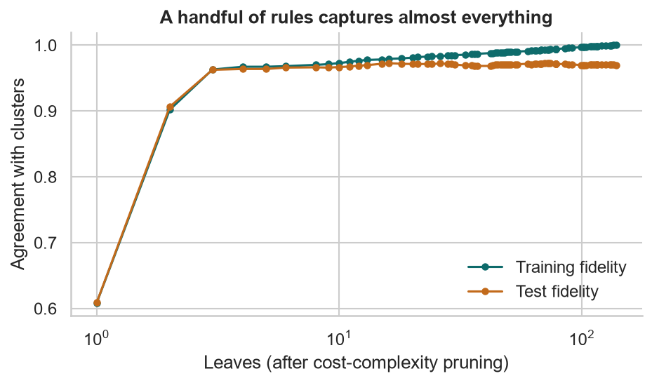
Going from 4 leaves to 138 buys 0.7 points of fidelity and costs all readability. For a manual, depth 2 is the sweet spot. An unlimited tree memorizes its training data (fidelity 1.000) and does no better on new members.
PruningCost-complexity pruning
$$R_\alpha(T) = R(T) + \alpha\,|T|$$
Grow a full tree, then remove the branches whose contribution is worth less than α per leaf.
path = DecisionTreeClassifier(random_state=0) \
    .cost_complexity_pruning_path(X_tr, y_tr)
for a in path.ccp_alphas:
    t = DecisionTreeClassifier(ccp_alpha=a, random_state=0)
    ...
Test fidelity barely moves between 4 and 138 leaves. Most of the structure is in the first two questions.
Human-Readable Rules
From a fitted tree to an underwriting manual.
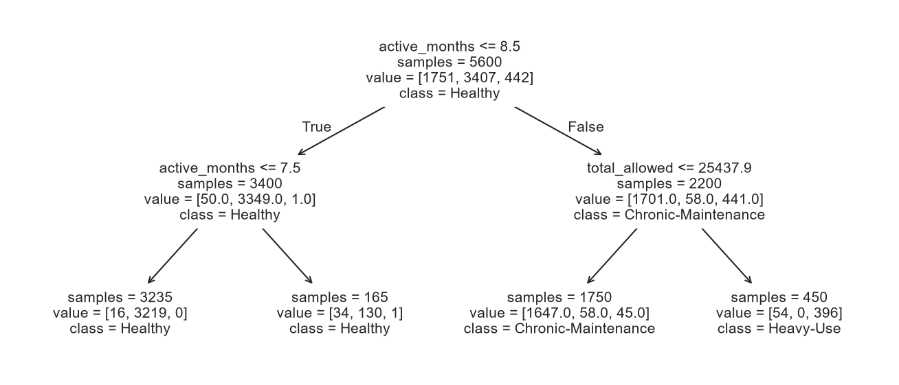
export_textThe whole model in nine lines
from sklearn.tree import export_text
print(export_text(tree, feature_names=list(feats.columns),
                  decimals=1, show_weights=True))
|--- active_months <= 8.5
| |--- active_months <= 7.5
| | |--- weights: [16.0, 3219.0, 0.0] class: Healthy
| |--- active_months > 7.5
| | |--- weights: [34.0, 130.0, 1.0] class: Healthy
|--- active_months > 8.5
| |--- total_allowed <= 25437.9
| | |--- weights: [1647.0, 58.0, 45.0] class: Chronic-Maintenance
| |--- total_allowed > 25437.9
| | |--- weights: [54.0, 0.0, 396.0] class: Heavy-UseWeights are training members per class: [Chronic-Maintenance, Healthy, Heavy-Use].
Both branches of the first split predict Healthy: the second split sharpens the probabilities but not the decision. A manual can merge them.
The manualThree rules, 96% agreement
Member risk tier — rules of assignment
- Care in 8 or fewer months of the year → Tier 1 · Preferred
- Care in 9 or more months and allowed cost up to $25,438 → Tier 2 · Care management
- Care in 9 or more months and allowed cost above $25,438 → Tier 3 · Complex care
Agrees with the clusters for 96.3% of members the tree never saw (5-fold CV of a depth-3 variant: 96.4%).
TIERS = {"Healthy": "Tier 1 · Preferred",
         "Chronic-Maintenance": "Tier 2 · Care management",
         "Heavy-Use": "Tier 3 · Complex care"}
tier = pd.Series(tree.predict(feats),
                 index=feats.index).map(TIERS)
These rules need a year of claims history, so they suit renewals and care management. For new applicants, grow the surrogate on features known at application time (age, conditions, prescriptions), and expect lower fidelity.
ValidationDo the tiers predict next year?
| Tier (from 2024) | Members | Mean 2024 | Mean 2025 | Relativity 2025 | Share of 2025 cost |
|---|---|---|---|---|---|
| 1 · Preferred | 4,863 | 1,581 | 3,874 | 0.35 | 21.4% |
| 2 · Care mgmt | 2,480 | 8,653 | 15,963 | 1.45 | 45.0% |
| 3 · Complex | 657 | 76,812 | 45,016 | 4.09 | 33.6% |
Members in the 30% test split only: 3,740 · 16,216 · 42,247. The tiers hold up on members the rules were not built from.
A Tier 3 member costs 11.6× a Tier 1 member the following year: 45,016 ÷ 3,874. That’s a rating variable, and a target list for a care-management program.
Tier 3’s cost falls from 76,812 to 45,016: regression to the mean again. Some complex-care members recover. Price and budget on the 2025 column, not the 2024 one.
InterpretabilityGlobal vs local explanations
Global (this lesson)
One small model explains the whole portfolio: “9+ active months and $25k+ means Tier 3”. Easy to audit, file, and teach.
Cost: fidelity. 3.75% of new members get a different answer than the clusters.
Local (Lesson 7)
Explain one prediction at a time from a complex model: “this driver’s rate is high because of age +0.29, sports car +0.28…” (SHAP).
Cost: no single rule book; explanations differ from policy to policy.
Regulators increasingly expect both: a rating plan you can describe, and an answer to “why did my premium go up?”
Actuarial Lab · 75 minAutomatic underwriting rules and risk tiers
- Rebuild the 2024 profiles and Lesson 5’s three named clusters
- Split 70/30, stratified by cluster
- Fit trees of depth 1–6 and unlimited; tabulate leaves and test fidelity
- Draw the cost-complexity pruning curve
- Export the depth-2 rules; write them as a three-line manual
- Map every member to a tier; compute 2025 cost, relativity, and cost share by tier
- Repeat step 6 on the test members only
Answer key
| Depth-2 test fidelity | 0.9625 |
| First split | active_months ≤ 8.5 |
| Second split | total_allowed ≤ 25,437.9 |
| Tier sizes | 4,863 · 2,480 · 657 |
| Tier 3 relativity (2025) | 4.09 |
RecapLesson 6 checklist
- I know why clusters need a surrogate to become rules
- I fit a surrogate tree on raw-unit features and measure test fidelity
- I control depth, leaf size, and pruning, and know the trade-off
- I export rules with
export_textand simplify them for a manual
- I map members to tiers and validate tiers on next year’s cost
- I watch for regression to the mean
- I know which features rules can use for new business vs renewals
- I can explain global vs local interpretability
Modern Non-Linear Modeling: Gradient Boosting & Trees
Back to the motor book: CART, random forests, XGBoost with a Poisson objective, and SHAP explanations.