Generalized Linear Models: Frequency & Count Models
The exponential dispersion family, Poisson regression with exposure offsets, overdispersion, and incidence rate ratios.
Lesson 2 · OverviewBy the end of this lesson you can…
- Describe the exponential dispersion family and the role of the link function
- Derive the Poisson GLM’s likelihood and its balance property
- Put policy exposure into a frequency model with an offset
- Diagnose overdispersion and fit a negative binomial model
- Interpret incidence rate ratios (IRRs) and their confidence intervals
- Choose between models with likelihood-ratio tests and AIC
Companion notebook: lesson-02-frequency-glms.ipynb — worked examples and self-checking exercises.
The dataLiability claims on the motor book
df = pd.read_parquet("data/processed/motor_model.parquet")
bins = [17, 21, 25, 30, 40, 50, 65, 75, 120]
labels = ["17-20", "21-24", "25-29", "30-39",
          "40-49", "50-64", "65-74", "75+"]
df["age_band"] = pd.cut(df["driver_age"], bins,
                        right=False, labels=labels)
df["log_miles"] = np.log(df["annual_mileage"] / 12_000)

train = df[df["policy_year"] <= 2024]   # fit on these
hold = df[df["policy_year"] == 2025]    # keep in the vault

train["n_liab"].value_counts()
# 0: 62,293 1: 3,579 2: 213 3: 12| Training (2021–24) | Holdout (2025) | |
|---|---|---|
| Vehicle-terms | 66,097 | 18,249 |
| Car-years | 63,815.9 | 8,964.6 |
| Liability claims | 4,041 | 524 |
| Frequency | 0.0633 | 0.0585 |
Policy year 2025 stays untouched until Lesson 7, when models compete on data none of them has seen.
One row per vehicle per policy term. exposure is car-years earned: a policy canceled after three months earns about 0.25.
One-way viewFrequency by driver age
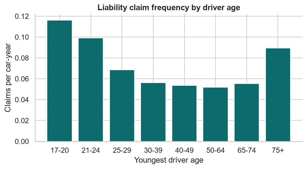
The familiar U: 0.116 for drivers aged 17–20, 0.052 at 50–64, 0.089 at 75+.
One-way tables mix effects. Young drivers are more likely to drive sports cars, so part of “young” is really “sports car”, and vice versa. A GLM estimates all factors at once, each adjusted for the others.
The GLM Framework
A distribution, a link, and a linear predictor.
EDFThe exponential dispersion family
$$f(y;\theta,\phi) = \exp\!\left(\frac{y\theta - b(\theta)}{\phi} + c(y,\phi)\right)$$
$$\mathrm{E}[Y] = \mu = b'(\theta) \qquad \mathrm{Var}(Y) = \phi\, V(\mu)$$
Each family is defined by its variance function V(μ): how the spread grows with the mean. φ is the dispersion.
| Family | V(μ) | Support | Actuarial use |
|---|---|---|---|
| Normal | 1 | ℝ | Rarely: symmetric errors |
| Poisson | μ | 0, 1, 2, … | Claim counts |
| Gamma | μ² | (0, ∞) | Severity (constant CV) |
| Inverse Gaussian | μ³ | (0, ∞) | Heavier-tailed severity |
| Tweedie | μp, 1 < p < 2 | {0} ∪ (0, ∞) | Pure premium |
Lesson 1’s CV table was a variance-function diagnostic: standard deviation ∝ mean means V(μ) ∝ μ², the Gamma.
LinkConnecting the mean to the predictors
$$g(\mu_i) = \eta_i = \mathbf{x}_i^\top\beta$$
- Random component: Yi from an EDF distribution with mean μi
- Systematic component: the linear predictor ηi
- Link: g maps the mean’s range onto the whole real line
With the log link, μ = eη is always positive and every coefficient is a multiplicative relativity:
$$\mu_i = e^{\beta_0}\,e^{\beta_1 x_{i1}}\cdots e^{\beta_p x_{ip}}$$
| Family | Canonical link | Used in pricing |
|---|---|---|
| Normal | identity | identity |
| Poisson | log | log |
| Gamma | inverse | log |
| Inverse Gaussian | 1/μ² | log |
| Tweedie | μ1−p | log |
Poisson Regression
Counts, exposure, and the offset.
TheoryThe Poisson GLM
$$P(Y_i = y) = \frac{e^{-\mu_i}\mu_i^{\,y}}{y!} \qquad \ln\mu_i = \mathbf{x}_i^\top\beta$$
Log-likelihood and its gradient (the score):
$$\ell(\beta) = \sum_i \big(y_i\,\mathbf{x}_i^\top\beta - e^{\mathbf{x}_i^\top\beta} - \ln y_i!\big)$$
$$\frac{\partial\ell}{\partial\beta} = \sum_i (y_i - \mu_i)\,\mathbf{x}_i = \mathbf{X}^\top(y-\mu) = 0$$
Solved by iteratively reweighted least squares (IRLS): usually 5–8 iterations.
Assumptions: claims arrive independently at a constant rate during the exposure period, and Var(Y) = E(Y).
The balance property. The intercept’s column is all ones, so its score equation says Σ yi = Σ μ̂i: fitted claims equal actual claims, in total and within every level of every categorical factor. A Poisson GLM can’t be “off” overall on its own training data.
ExposureOffsets: modeling a rate, not a count
A vehicle insured for half a year should expect half the claims:
$$\mu_i = \text{Exposure}_i \times e^{\mathbf{x}_i^\top\beta} \iff \ln\mu_i = \ln(\text{Exposure}_i) + \mathbf{x}_i^\top\beta$$
ln(Exposure) enters the linear predictor with its coefficient fixed at 1. It’s an offset, not a feature.
import statsmodels.api as sm
import statsmodels.formula.api as smf

pois = smf.glm("n_liab ~ " + rhs, data=train,
               family=sm.families.Poisson(),
               offset=np.log(train["exposure"])).fit()

# identical: statsmodels takes the log for you
smf.glm(..., exposure=train["exposure"])
Three wrong ways to handle exposure:
- Ignore it: a one-week policy counts like a full year
- Add exposure as a feature: the model estimates a coefficient that should be fixed
- Model n/exposure with OLS: back to all of Lesson 1’s problems
With the offset, eβ is a ratio of claims per car-year, the frequency, however long each policy was on the books.
FitThe full frequency model
rhs = ("C(vehicle_style, Treatment('Sedan'))"
       " + C(age_band, Treatment('40-49'))"
       " + urban + log_miles"
       " + C(channel, Treatment('Agent'))"
       " + holder_gender")
pois = smf.glm("n_liab ~ " + rhs, data=train,
               family=sm.families.Poisson(),
               offset=np.log(train["exposure"])).fit()

irr = np.exp(pois.params)
ci = np.exp(pois.conf_int())
pois.fittedvalues.sum()      # 4,041.00 = actual claims
Deviance 22,430.1 on 66,079 df · AIC 30,216.8
| Term | IRR | 95% CI | p |
|---|---|---|---|
| Sports (vs Sedan) | 1.728 | 1.547–1.930 | <0.001 |
| SUV | 1.223 | 1.126–1.330 | <0.001 |
| Minivan | 0.855 | 0.736–0.994 | 0.041 |
| Age 17–20 (vs 40–49) | 2.059 | 1.838–2.307 | <0.001 |
| Age 75+ | 1.680 | 1.456–1.938 | <0.001 |
| Urban | 1.366 | 1.280–1.459 | <0.001 |
| log_miles | 1.630 | 1.522–1.746 | <0.001 |
| Channel: Broker | 0.987 | 0.900–1.082 | 0.781 |
| Channel: Direct | 0.966 | 0.903–1.032 | 0.304 |
| Gender: M | 1.025 | 0.964–1.090 | 0.430 |
SelectionWhich factors earn their place?
Likelihood-ratio test: drop channel and gender
lr = 2 * (full.llf - reduced.llf)      # 1.703
df_diff = reduced.df_resid - full.df_resid   # 3
scipy.stats.chi2.sf(lr, df_diff)       # p = 0.636
full.aic, reduced.aic                  # 30,216.8 → 30,212.5
No evidence that channel or gender affects frequency, and the truth agrees: neither was used to simulate claims. Drop them.
Age as a straight line?
Replace the bands with driver_age: one coefficient, IRR 0.925 per decade — “older is safer”, which is wrong for everyone over 70.
| Age specification | AIC |
|---|---|
| Linear in age | 30,417.1 |
| Eight bands | 30,212.5 |
AIC = −2 log-likelihood + 2 × parameters. Lower is better, and it penalizes extra parameters. A GLM is linear in the predictor; shapes like the U need bands, splines, or transformations you choose.
Overdispersion
When Var(Y) > E(Y).
OverdispersionWhen counts are more variable than Poisson
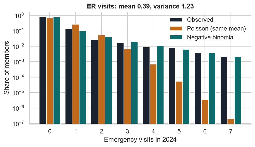
Emergency visits per health member in 2024: mean 0.395, variance 1.227, three times the mean.
- Poisson predicts 67% zeros; observed 79%
- Poisson says 5+ visits is almost impossible; 1.9% of members had them
The usual cause is unobserved heterogeneity: members (or drivers) differ in ways the features don’t capture. A mixture of Poissons with different rates is overdispersed.
Diagnose & fixNegative binomial regression
$$\text{NB2:}\quad \mathrm{Var}(Y) = \mu + \alpha\mu^2$$
Gamma-distributed rate multipliers with variance α. α = 0 is the Poisson.
# Diagnose: Pearson chi-square per degree of freedom
pois.pearson_chi2 / pois.df_resid      # 1.049

# Estimate alpha by maximum likelihood
nb = smf.negativebinomial("n_liab ~ " + rhs2, data=train,
        offset=np.log(train["exposure"])).fit()
nb.params["alpha"]                     # 0.649 (se 0.110)
2 * (nb.llf - pois.llf) # LR = 50.4| Evidence | Value |
|---|---|
| Pearson χ²/df, vehicle-term level | 1.049 |
| Pearson χ²/df, policyholder level | 1.147 |
| NB α (standard error) | 0.649 (0.110) |
| AIC Poisson → NB | 30,212.5 → 30,164.0 |
The book was simulated with a gamma “driver quality” factor of variance 0.83, and the NB found it. At a frequency of 0.06, α matters little for one policy-year (dispersion ≈ 1 + 0.06α) but a lot for multi-year experience and for experience rating.
ConsequencesSame relativities, honest standard errors
| Term | Poisson IRR | NB IRR | Poisson SE | NB SE |
|---|---|---|---|---|
| Sports | 1.728 | 1.720 | 0.0564 | 0.0583 |
| Age 17–20 | 2.062 | 2.059 | 0.0581 | 0.0600 |
| Age 75+ | 1.680 | 1.679 | 0.0729 | 0.0749 |
| Urban | 1.365 | 1.365 | 0.0334 | 0.0341 |
| log_miles | 1.629 | 1.629 | 0.0351 | 0.0360 |
- Poisson estimates stay consistent under overdispersion: the mean model is still right
- Its standard errors are too small, so its p-values are too optimistic
- Here the difference is 2–4%. On health visit counts (variance 3–6× the mean) it would be huge
A lighter alternative: keep the Poisson fit and scale its SEs by √(Pearson χ²/df) — the quasi-Poisson approach, .fit(scale="X2").
Incidence Rate Ratios
Reading a frequency model like a rating manual.
InterpretationWhat an IRR says
| Term | IRR | Plain English |
|---|---|---|
| Urban | 1.365 | Urban-garaged cars have 36.5% more liability claims per car-year, other factors equal |
| Age 17–20 | 2.062 | Twice the frequency of a 40–49 driver in the same car and place |
| Minivan | 0.856 | 14% fewer claims than a sedan |
| log_miles | β = 0.489 | An elasticity: 10% more miles → 1.10.489 = +4.8%; double the miles → +40% |
IRRs multiply. A 19-year-old in an urban sports car driving 15,000 miles:
2.062 × 1.728 × 1.365 × 1.250.489 = 5.42× the base rate
“Other factors equal” is doing real work. An IRR is the effect adjusted for everything else in the model, and only for what’s in the model.
CheckFitted relativities vs the truth
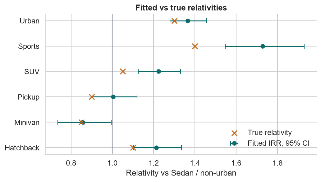
- Urban (truth 1.30) and Minivan (0.85) sit inside their intervals
- Every style is measured against Sedan, and in this sample Sedans ran 7% below their true expected claims — about two standard errors. A noisy base level shifts every contrast
Sports: 1.73 vs a truth of 1.40. The book has an interaction the model doesn’t contain: young drivers in sports cars claim an extra 60%. With no term for it, the model spreads that effect over Sports and the young age bands. Lesson 7 shows how to find it.
Actuarial Lab · 75 minA motor claim frequency model
- Load
motor_model.parquet; addage_bandandlog_miles; keep policy years ≤ 2024 - One-way frequencies by age band, style, urban, channel
- Fit the full Poisson GLM with a log(exposure) offset; confirm the balance property
- LR-test channel and gender; refit without them
- Compare banded age with linear age by AIC
- Pearson χ²/df, then a negative binomial; compare IRRs and SEs
- Build an IRR table with 95% intervals and compare it with the truth
Answer key: reduced Poisson model
| Term | IRR | Truth |
|---|---|---|
| Base frequency | 0.0397 | — |
| Age 17–20 | 2.062 | 1.957 |
| Age 21–24 | 1.767 | 1.484 |
| Age 25–29 | 1.279 | 1.173 |
| Age 75+ | 1.680 | 1.631 |
| Urban | 1.365 | 1.30 |
| Mileage elasticity β | 0.489 | 0.50 |
True age relativities are exposure-weighted averages of the smooth curve within each band.
RecapLesson 2 checklist
- I can name a GLM’s three parts: distribution, link, linear predictor
- I know each family by its variance function
- I model frequency with a Poisson GLM and a log(exposure) offset
- I check that fitted claims balance to actual claims
- I drop factors with LR tests and AIC, not gut feel
- I test for overdispersion and know when NB matters
- I read IRRs as adjusted multiplicative effects
- I know a missing interaction bends the factors that are in the model
GLMs: Severity & Pure Premium Modeling
Gamma and inverse Gaussian severity models, the frequency × severity pure premium, and the Tweedie.