Statistical Foundations of Predictive Modeling
Ordinary least squares, why it breaks on insurance data, and the log link that every pricing model in this course is built on.
Lesson 1 · OverviewBy the end of this lesson you can…
- Place an actuarial problem in the supervised or unsupervised paradigm
- State the Gauss–Markov assumptions and check them with residual plots
- Explain why skewness, zeros, and non-constant variance break OLS on insurance data
- Fit a log-linear model in
statsmodelsand read its coefficients as multiplicative relativities - Correct the retransformation bias when you go back from log-dollars to dollars
- Use heteroscedasticity-consistent standard errors (
HC0,HC3)
Companion notebook: lesson-01-statistical-foundations.ipynb — worked examples and self-checking exercises.
Course 3Two books of business
Motor book · data/motor/
- Same six-table schema as Course 2, five policy years (2021–2025)
- 84,346 vehicle-terms · 72,781 car-years · 4,565 liability claims
- Ready-to-model frame:
data/processed/motor_model.parquet - Lessons 2, 3, 7, 8: frequency, severity, pure premium, boosting
Health book · data/health/
- 8,000 members, 375,810 encounters in 2024–2025
- Eight service categories, from lab tests to inpatient stays
- Wellness screening results and a lifestyle survey
- Lessons 1, 4, 5, 6: severity, regularization, clustering, rules
Both books are simulated from a known risk model. Real data never tells you whether your model found the truth; these books do. Throughout the course, you’ll check fitted relativities against the values that generated the data.
Supervised & Unsupervised
Two ways to learn from a portfolio.
ParadigmsWhat are you trying to learn?
| Paradigm | Has a target? | Insurance examples | Lessons |
|---|---|---|---|
| Supervised · regression | Yes, a number | Claim frequency, severity, pure premium, reserves | 1–4, 7, 8 |
| Supervised · classification | Yes, a label | Will this policy lapse? Is this claim fraudulent? Which tier? | 6 |
| Unsupervised · clustering | No | Patient archetypes, driver segments, territory groupings | 5 |
| Unsupervised · anomaly | No | Unusual billing patterns, data-quality outliers | — |
Supervised learning fits f(features) ≈ target on examples where the answer is known, then predicts it for new risks.
Unsupervised learning finds structure — groups, directions, outliers — in features alone. Its output must still be interpreted and validated.
WorkflowEvery model in this course follows the same path
Most modeling mistakes happen before the first .fit(): the wrong target (loss ratio instead of pure premium), the wrong exposure, or a feature that leaks the answer.
This lesson is about the Fit box: what the classical linear model assumes, and what to do when insurance data refuses to cooperate.
The Classical Linear Model
OLS, its assumptions, and how to check them.
OLSOrdinary least squares
$$y = \mathbf{X}\beta + \varepsilon \qquad \hat\beta = (\mathbf{X}^\top\mathbf{X})^{-1}\mathbf{X}^\top y$$
OLS picks the β that minimizes the sum of squared residuals $\sum_i (y_i - \mathbf{x}_i^\top\beta)^2$.
Gauss–Markov assumptions
- Linearity — E[y] is linear in the parameters
- Full rank — no feature is an exact combination of others
- Exogeneity — E[ε | X] = 0
- Homoscedasticity — Var(ε | X) = σ², the same for every row
- No autocorrelation — errors are uncorrelated
Under 1–5, OLS is BLUE: the Best (minimum-variance) Linear Unbiased Estimator. Add normal errors and the t-tests and confidence intervals are exact.
Assumption 4 is the one insurance data breaks first. When it fails, the coefficients are still unbiased — but the standard errors are wrong, and so is every p-value built on them.
statsmodelsFitting OLS with a formula
import statsmodels.formula.api as smf

enc = pd.read_parquet("data/health/encounters.parquet")
mem = pd.read_csv("data/health/members.csv")
e = (enc[enc["service_date"].dt.year == 2024]
     .merge(mem, on="member_id", validate="many_to_one"))
e["age10"] = (e["age"] - 40) / 10     # decades from age 40

rhs = ("C(service_category, Treatment('Office Visit'))"
       " + age10 + C(region, Treatment('Suburban'))"
       " + C(plan, Treatment('PPO'))")
ols = smf.ols("allowed ~ " + rhs, data=e).fit()
ols.rsquared          # 0.461
ols.params["age10"] # 30.7 dollars per decade- 180,472 encounters from 2024, one row each
C(col, Treatment('level'))makes dummy variables and names the base level- Coefficients are additive dollars: an inpatient stay adds $37,722 to the base; a Metro member adds $94.50 to every encounter, from a $55 lab test to a $30,000 admission
An R² of 0.46 looks respectable. The residuals tell a different story.
DiagnosticsRead the residuals, not the R²
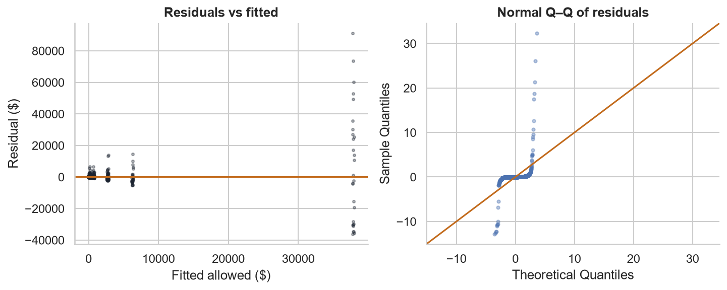
- Fan shape: residual spread grows with the fitted value — heteroscedasticity
- Q–Q tails: residuals reach 30 standard deviations — far from normal
- 3,810 negative fitted values (as low as −$107.51) for costs that can never be negative
- Additive effects: an HMO discount of $56.80 whether the claim is a lab test or a surgery
Why OLS Breaks on Insurance Data
Skewness, zeros, and variance that grows with the mean.
Problem 1Positive skewness
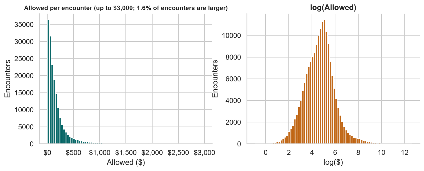
Mean $441.14 vs median $111.48 · skewness 34.3 · only 11.1% of encounters exceed the mean · largest $303,889
When the mean sits at the 89th percentile, a model of the mean is driven by a handful of large claims. On the log scale the same data is close to symmetric.
Problem 2Zeros and concentration
| Book | Statistic | Value |
|---|---|---|
| Motor | Vehicle-terms with no liability claim | 94.2% |
| Health | Members with zero 2024 cost | 0.8% |
| Health | Share of 2024 cost from the top 10% of members | 68.6% |
A normal distribution puts no probability on an exact zero, and is symmetric. Aggregate loss per policy is usually zero — and occasionally enormous.
Two fixes you’ll meet in this course:
- Split the problem — model how often (frequency, Lesson 2) and how much (severity, Lesson 3) separately
- Use a distribution with a mass at zero — the Tweedie, Lesson 3
Problem 3Variance grows with the mean
| Category | Mean | Std dev | CV |
|---|---|---|---|
| Lab | 79 | 67 | 0.85 |
| Office Visit | 167 | 68 | 0.40 |
| Pharmacy | 169 | 324 | 1.92 |
| Specialist | 338 | 175 | 0.52 |
| Imaging | 703 | 743 | 1.06 |
| Emergency | 2,728 | 2,440 | 0.89 |
| Outpatient Surgery | 6,282 | 4,804 | 0.76 |
| Inpatient | 37,895 | 40,879 | 1.08 |
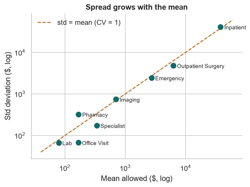
The standard deviation is roughly proportional to the mean (a constant coefficient of variation) — nothing like OLS’s single σ².
The Log Transformation
From additive dollars to multiplicative rating factors.
Log-linearModel log(cost): effects become multipliers
$$\ln y = \beta_0 + \beta_1 x_1 + \dots + \varepsilon \;\Longrightarrow\; y = e^{\beta_0}\cdot e^{\beta_1 x_1}\cdots e^{\varepsilon}$$
e["log_allowed"] = np.log(e["allowed"])
loglin = smf.ols("log_allowed ~ " + rhs, data=e).fit()

rel = np.exp(loglin.params)     # relativities
loglin.rsquared                 # 0.397
np.sqrt(loglin.scale) # residual sd 1.019- eβ is a relativity: Metro costs 1.163× Suburban, for every kind of encounter
- This is exactly how rating plans work: base rate × factor × factor × …
| Term | Fitted | HC3 95% CI | Truth |
|---|---|---|---|
| Region: Metro | 1.163 | 1.150–1.175 | 1.15 |
| Region: Rural | 0.899 | 0.887–0.910 | 0.90 |
| Plan: HMO | 0.874 | 0.865–0.883 | 0.88 |
| Plan: HDHP | 0.977 | 0.964–0.989 | 0.97 |
| Age, per decade | 1.058 | 1.054–1.062 | 1.06 |
| Emergency vs Office | 12.9 | 12.6–13.3 | — |
| Inpatient vs Office | 151.7 | 141.8–162.2 | — |
Category relativities have no single “truth”: heavy users’ encounters are more intensive, and the mix differs by category.
PitfallThe retransformation problem
$$e^{\,\mathrm{E}[\ln y]} \neq \mathrm{E}[y] \qquad \text{for lognormal errors: } \mathrm{E}[y] = e^{\mathbf{x}^\top\beta + \sigma^2/2}$$
np.exp(fitted) estimates the median, not the mean. Duan’s smearing estimator multiplies by the average of eresidual:
naive = np.exp(loglin.fittedvalues)
smear = np.mean(np.exp(loglin.resid))          # 1.755

# heteroscedastic? smear within each category
cat = (e.assign(r=np.exp(loglin.resid))
        .groupby("service_category")["r"].mean())
fixed = naive * e["service_category"].map(cat)| Mean allowed | Actual | Naive | One smear | By category |
|---|---|---|---|---|
| Pharmacy | 168.6 | 77.3 | 135.6 | 168.7 |
| Office Visit | 167.4 | 156.8 | 275.1 | 167.4 |
| Emergency | 2,727.9 | 2,053.7 | 3,603.9 | 2,719.3 |
| Inpatient | 37,894.9 | 24,019.7 | 42,150.2 | 37,735.9 |
| All | 441.1 | 292.5 | 513.3 | 440.2 |
The naive retransform understates total cost by a third. One global smearing factor overshoots because the residual variance differs by category. A pricing model has to get the mean right.
PreviewLog transformation vs log link
Log-linear OLS (this lesson)
$$\mathrm{E}[\ln y] = \mathbf{x}^\top\beta$$
- Models the mean of log-cost
- Needs a retransformation to get dollars
- Can’t handle zeros: ln 0 = −∞
GLM with a log link (Lessons 2–3)
$$\ln \mathrm{E}[y] = \mathbf{x}^\top\beta$$
- Models the mean in dollars directly — no smearing
- Keeps multiplicative relativities: Gamma log-link GLM gives Metro 1.175, HMO 0.878
- Chooses a variance function to match the data
The log link is the backbone of modern pricing: multiplicative rating factors, predictions that are always positive, and a mean that’s right in dollars.
Robust Standard Errors
Honest uncertainty when the variance isn’t constant.
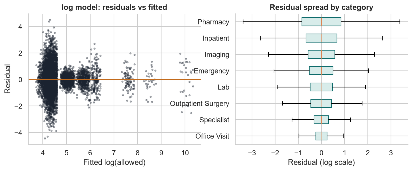
HeteroscedasticityThe log model still has it
from statsmodels.stats.diagnostic import het_breuschpagan
lm, p, *_ = het_breuschpagan(loglin.resid, loglin.model.exog)
# LM = 21,147.6, p < 1e-300
Residual standard deviation runs from 0.36 for office visits to 1.25 for pharmacy (generics next to specialty drugs). The Breusch–Pagan test rejects constant variance emphatically.
Sandwich estimatorsHC0 and HC3
$$\widehat{\mathrm{Var}}(\hat\beta) = (\mathbf{X}^\top\mathbf{X})^{-1}\,\Big(\sum_i \omega_i\,\hat e_i^2\,\mathbf{x}_i\mathbf{x}_i^\top\Big)\,(\mathbf{X}^\top\mathbf{X})^{-1}$$
- HC0 (White): ωi = 1 — each row’s own squared residual
- HC3: ωi = 1 / (1 − hii)² — inflates high-leverage rows; better in small samples
hc3 = smf.ols("log_allowed ~ " + rhs, data=e).fit(cov_type="HC3")
np.exp(hc3.conf_int()) # robust 95% CIs for the relativities| Std error | OLS | HC0 | HC3 |
|---|---|---|---|
| Specialist | 0.0107 | 0.0045 | 0.0045 |
| Lab | 0.0088 | 0.0049 | 0.0049 |
| Inpatient | 0.0360 | 0.0342 | 0.0343 |
| Region: Metro | 0.0054 | 0.0054 | 0.0054 |
| Age per decade | 0.0020 | 0.0020 | 0.0020 |
Robust SEs are correct, not automatically bigger. Here the base level (office visits) is unusually tight, so category contrasts get smaller SEs. Region, plan, and age hardly move.
Actuarial Lab · 75 minBaseline severity by service category
- Load the 2024 encounters, join member age, region, and plan
- Fit OLS on raw allowed; list three things the residual plots tell you
- Fit the log-linear model; tabulate relativities with HC3 95% intervals
- Run Breusch–Pagan; compare OLS, HC0, and HC3 standard errors
- Compute category-level smearing factors
- Predict the median and mean allowed per encounter for a reference member: age 40, Suburban, PPO
- Compare region, plan, and age relativities with the truth
Answer key: reference member
| Category | Median | Mean |
|---|---|---|
| Lab | 59.10 | 76.17 |
| Pharmacy | 74.10 | 161.83 |
| Office Visit | 151.94 | 162.21 |
| Specialist | 288.93 | 322.24 |
| Imaging | 466.39 | 671.65 |
| Emergency | 1,963.74 | 2,600.17 |
| Outpatient Surgery | 4,815.04 | 5,986.45 |
| Inpatient | 23,045.56 | 36,205.44 |
Pharmacy’s mean is more than twice its median: the widest spread of any category.
RecapLesson 1 checklist
- I can say whether a problem is supervised or unsupervised
- I can list the Gauss–Markov assumptions and what breaks when each fails
- I read residual-vs-fitted and Q–Q plots before I read R²
- I know why skew, zeros, and mean-dependent variance defeat OLS
- I read eβ from a log model as a multiplicative relativity
- I correct retransformation bias with (category-level) smearing
- I use
cov_type="HC3"when variance isn’t constant - I know the difference between a log transform and a log link
GLMs for Claim Frequency
The exponential family, Poisson regression with exposure offsets, overdispersion, and incidence rate ratios, on the motor book.