Python for Actuarial Students · Course 4

Lesson 3

Stochastic Simulation & Performance

A Monte Carlo asset-liability model for an annuity book: reproducible random numbers, profiling, vectorization, and compiled loops with numba, all the way to economic capital from a million scenarios.

Lesson 3 · OverviewBy the end of this lesson you can…

Project annuity cash flows under stochastic interest and mortality
Manage seeds so every run, serial or parallel, can be reproduced
Find the slow part with cProfile and line_profiler before optimizing
Replace Python loops with NumPy array operations, and know their memory cost
Compile loops with numba and run scenarios in parallel
Estimate economic capital, and its sampling error, for two asset strategies

75 min

Concepts & worked examples

75 min

Lab: a million-scenario ALM run

Companion notebook: lesson-03-simulation-performance.ipynb — worked examples and self-checking exercises.

The problemAn annuity book and the assets behind it

In-force immediate annuities
Annuitants	5,000, ages 60–100 (mean 72.6)
Payments	$69.4m a year, at each year end while alive
Reserve at 4%	$762.2m (10.98 years of payments)
Horizon	60 years: the youngest reaches 120

Mortality: the Standard Ultimate Survival Model, μ_x = A + Bc^x (A = 0.00022, B = 2.7×10⁻⁶, c = 1.124). First check: ä₆₅ at 5% = 13.5498, the textbook value.

What can go wrong, one draw per scenario:

Interest: a Vasicek short rate, r₀ = 3%, reverting to 4% at speed 0.10, volatility 1%
Longevity trend: mortality improves by g a year, g ~ N(1.5%, 0.75%)
Who dies when: one uniform U per life; it is paid until the first year its survival probability falls below U

Economic capital: what covers the liabilities’ cost in all but the worst 1 scenario in 200, above the average cost.

One scenarioFrom draws to a present value

# rates: exact annual Vasicek steps
e = math.exp(-a)
sd = sigma * math.sqrt((1 - e * e) / (2 * a))
r[:, t] = r[:, t - 1] * e + b * (1 - e) + sd * z[:, t]

# discount factor for a payment at the end of year t
D = np.exp(-np.cumsum(r, axis=1))
C = np.cumsum(D, axis=1)          # C[k] = D_1 + ... + D_k

# a life aged x survives t years with probability S_x(t);
# it receives K payments, K = max{t : S_x(t) > U}
pv = sum(payment[i] * C[K[i]] for i in lives)

Each scenario is a full 60-year projection of 5,000 lives: 300,000 life-years, and one present value at the end.

Scenario 0 of the test set: $890,175,321.12, above the $762m reserve because rates start at 3%, not 4%.

The trick for speed: C(k) turns “sum the discounted payments” into one lookup per life, and the survival curve depends only on age, so compute 41 curves, not 5,000.

Part 1

Reproducible Randomness

A result you can’t reproduce can’t be audited.

SeedsOne generator, one seed, every draw

rng = np.random.default_rng(2026)          # a Generator
z  = rng.standard_normal((n, 60))          # rates
zg = rng.standard_normal(n)                # longevity
u  = rng.random((n, 5_000))                # lives

# parallel work: independent child streams
children = np.random.SeedSequence(2026).spawn(8)
rngs = [np.random.default_rng(s) for s in children]

Never the global np.random.seed: any library call can move it
Store the seed with the results, as you would the data version
SeedSequence.spawn gives streams that don’t overlap, so workers never share numbers

In parallel code, which thread runs which scenario changes from run to run. The model on the next slides seeds each scenario from seed + s, so the answer doesn’t depend on the thread count: 2 threads and 6 threads give identical results.

Part 2

Making It Fast

Measure, then fix the part that matters.

Profile firstThe legacy model: 5.4 scenarios a second

992244 function calls in 0.586 seconds

 ncalls  tottime  cumtime  function
 198281    0.373    0.409  alm.py:83(legacy_q)
      1    0.136    0.586  alm.py:89(legacy_pv)
 396673    0.035    0.035  {built-in method math.exp}
 198403    0.023    0.023  {method 'random' ...}
 198333    0.018    0.018  {built-in method math.log}

 Hits   % Time  Line Contents
38993     7.2   df *= math.exp(-rates[t - 1])
38993    78.8   if rnd.random() < legacy_q(age + t - 1,
                                           t, g, ...):
36993     7.3   pv += pay * df

The legacy model recomputes q_x from the Makeham formula 198,281 times for two scenarios, the same 60 ages over and over. 79% of the time is on one line.

Guessing where the time goes is usually wrong. cProfile says which function; line_profiler says which line.

SpeedFour versions, same answer

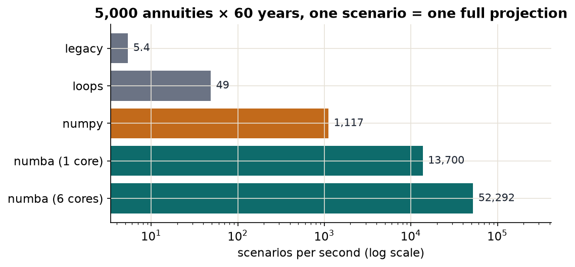
Scenarios per second on a log scale: legacy 5.4, loops 49, NumPy 1,117, numba one core 13,700, numba six cores 52,292

Version	Idea	vs legacy
loops	precomputed survival tables	×9
NumPy	all lives at once, per scenario	×208
numba, 1 core	compiled loops	×2,547
numba, 6 cores	`prange` over scenarios	×9,723

On the same random numbers, the versions agree to $0.000005 on present values near $900m. Always test that a fast version gives the slow version’s answer.

VectorizationNo Python loop over lives

uniq, idx = np.unique(ages, return_inverse=True)   # 41 ages

for lo in range(0, n, chunk):          # 100 scenarios at a time
    S = np.stack([survival(q, uniq, g)[:, 1:]
                  for g in g_chunk])    # (100, 41, 60)
    K = (S[:, idx, :] > u[lo:hi, :, None]).sum(axis=2)
    pv[lo:hi] = (payments *
                 np.take_along_axis(C[lo:hi], K, axis=1)).sum(axis=1)

Broadcasting compares every life with every year in one step: 100 × 5,000 × 60 booleans per chunk.

Vectorization spends memory to save time. One chunk of 100 scenarios is 30 MB of booleans; a million scenarios at once would be 300 GB. Chunk, or move to compiled loops that need almost no memory.

numbaWrite the loop; let the compiler make it fast

import numba as nb

@nb.njit(parallel=True, cache=True)
def simulate(q, uniq, idx, payments, n, seed, r0, a, b,
             sigma, g_mean, g_sd, cf_expected):
    pv = np.empty(n)
    for s in nb.prange(n):              # scenarios in parallel
        np.random.seed(seed + s)        # one seed per scenario
        g = g_mean + g_sd * np.random.standard_normal()
        S = _survival_nb(q, uniq, g)    # 41 curves
        ...                              # rates, C(k)
        total = 0.0
        for i in range(len(idx)):       # plain loops: fine here
            uu = np.random.random()
            k = 0
            while k < T and S[idx[i], k + 1] > uu:
                k += 1
            total += payments[i] * C[k]
        pv[s] = total
    return pv

@njit compiles the function to machine code on first call (1.6 s here); cache=True keeps it for next time
Only NumPy arrays, numbers, and simple loops inside: no pandas, no dicts of objects
prange splits scenarios across cores; each scenario writes only its own pv[s]
Memory: a few kilobytes per thread, whatever n is

Order of attack: profile → better algorithm (precompute) → NumPy → numba. Most code stops at step 2 or 3.

Part 3

Economic Capital

What the speed buys.

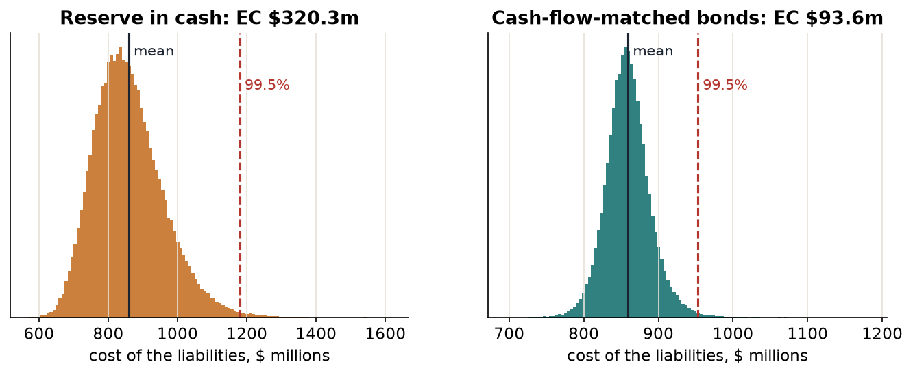
ALMTwo ways to hold the reserve

Cash: the assets earn the short rate, year by year. The cost of the liabilities is their PV along the scenario’s rate path.
Cash-flow matched: at time 0, buy zero-coupon bonds paying the best-estimate cash flows. Only the difference between actual and expected payments is exposed to rates.

Cost (matched) = bond price + PV(actual) − PV(expected)

EC = 99.5th percentile of cost − mean cost

Histograms of the cost of the liabilities over 100,000 scenarios: reserve in cash, spread from about 600 to 1,300 million, EC 320.3 million; cash-flow matched, narrow around 860 million, EC 93.6 million

ResultsHow many scenarios are enough?

Scenarios	Run time	EC, cash	EC, matched
10,000	1.5 s	$319.5m	$90.6m
100,000	3.1 s	$320.3m	$93.6m
1,000,000	30.4 s	$325.7m	$94.7m

Best-estimate cost $859.6m. Ten batches of 100,000 give cash EC with a standard deviation of $2.5m: at 100,000 scenarios the 99.5th percentile rests on the worst 500.

Only this risk switched on	EC, cash
Interest rates	$301.6m
Longevity trend	$76.2m
Who dies when (5,000 lives)	$13.9m

Matching the cash flows removes most of the interest-rate risk and cuts capital from $326m to $95m. What’s left is longevity, which no bond portfolio hedges. Capital estimates need their own error bars.

Actuarial Lab · 75 minA million-scenario ALM run

Build the Makeham q_x table; check ä₆₅ at 5% = 13.5498; reserve at 4%
Vasicek paths from a seeded Generator; discount factors; P(0, 10)
Profile the legacy model; name the hot spot
A vectorized version that matches the loop version exactly
A numba version; time all three; check they agree
EC for cash and matched strategies; repeat at 10k, 100k, 1m scenarios
Batch the million run to estimate the EC’s standard error

Answer key

ä₆₅ at 5%	13.5498
Reserve at 4%	$762,202,760
Hot spot	`legacy_q`
EC, 1m scenarios: cash	$325.7m
… matched	$94.7m
Batch s.d. of cash EC	$2.5m

RecapLesson 3 checklist

My simulation reproduces a deterministic textbook value
Every random number comes from a seeded Generator
Parallel results don’t depend on the thread count
I profile before I optimize

I vectorize, and I know what it costs in memory
I compile hot loops with numba when NumPy isn’t enough
Every fast version is tested against the slow one
I report capital with its sampling error

Up next

Lesson 4

Actuarial APIs with FastAPI

The Course 3 champion model behind an HTTP API: request and response schemas, validation, authentication, OpenAPI documentation, and what async does and doesn’t buy.

← Course home Next: Lesson 4 →