Unsupervised Learning & Risk Group Discovery
No target and no labels: turning 180,000 health encounters into member profiles, then letting K-means find the patient archetypes.
Lesson 5 · OverviewBy the end of this lesson you can…
- Contrast clustering with regression: what “right” means without a target
- Aggregate multi-encounter data into one behavioral profile per member
- Explain the K-means algorithm, its distance metric, and the curse of dimensionality
- Transform and scale features so distances mean something
- Choose k with the elbow method and silhouette scores
- Translate clusters into business language with z-score heatmaps and radar charts
Companion notebook: lesson-05-clustering.ipynb — worked examples and self-checking exercises.
Learning Without a Target
What clustering is for, and what it can’t do.
TheoryClustering vs regression
| Regression (Lessons 1–4) | Clustering (this lesson) | |
|---|---|---|
| Input | Features and a target | Features only |
| Goal | Predict the target | Group similar rows |
| “Correct” means | Low error on new data | Groups that are compact, separated, and useful |
| Validation | Holdout score | Internal indices + business judgment |
| Output | A number per row | A label per row + group profiles |
Why cluster members at all?
- Care-management programs need target populations
- Underwriters need a small number of recognizable risk groups
- Pricing can use cluster membership as a rating variable
K-means will always return k clusters, even from pure noise. Finding groups is easy; finding groups that are real and meaningful is the work.
Feature Engineering for Clustering
From encounters to one row per member.
AggregationMany encounters → one static profile
enc = pd.read_parquet("data/health/encounters.parquet")
mem = pd.read_csv("data/health/members.csv")
e = enc[enc["service_date"].dt.year == 2024]

counts = e.pivot_table(index="member_id",
                       columns="service_category",
                       values="encounter_id",
                       aggfunc="count", fill_value=0)
counts.columns = [c.lower().replace(" ", "_")
                  for c in counts.columns]
prof = counts.reindex(mem["member_id"], fill_value=0)

prof["total_allowed"] = (e.groupby("member_id")["allowed"]
                          .sum().reindex(prof.index, fill_value=0))
prof["active_months"] = (e.assign(m=e["service_date"].dt.month)
                          .groupby("member_id")["m"].nunique()
                          .reindex(prof.index, fill_value=0))
180,472 encounters in 2024, 22.6 per member, become an 8,000 × 10 table:
| Feature | Mean | Median | Max |
|---|---|---|---|
| office_visit | 3.30 | 2 | 33 |
| pharmacy | 12.73 | 4 | 133 |
| emergency | 0.39 | 0 | 15 |
| inpatient | 0.10 | 0 | 7 |
| total_allowed | 9,952 | 1,714 | 421,889 |
| active_months | 7.07 | 6 | 12 |
reindex keeps members with no encounters: they’re a real (healthy) group, not missing data.
Transform & scaleMake distances mean something
from sklearn.preprocessing import StandardScaler
X = StandardScaler().fit_transform(np.log1p(prof))- log1p tames the skew: one member with 133 fills shouldn’t define the pharmacy axis
- Standardize so each feature has mean 0, sd 1. Otherwise total_allowed (sd $27,718) outweighs everything measured in counts
| Preparation | Cluster sizes | Agreement with truth (ARI) |
|---|---|---|
| Raw values | 7,501 · 420 · 79 | 0.178 |
| Standardized | 5,004 · 2,438 · 558 | 0.918 |
| log1p + standardized | 4,868 · 2,501 · 631 | 0.926 |
ARI (adjusted Rand index) compares two labelings: 1 = identical, 0 = chance. We can compute it only because this book was simulated from known archetypes; real data never gives you this.
K-Means
Centroids, distances, and dimensions.
AlgorithmLloyd’s algorithm
$$\min_{C_1,\dots,C_k}\;\sum_{j=1}^{k}\sum_{i\in C_j}\lVert \mathbf{x}_i - \boldsymbol{\mu}_j\rVert^2$$
- Place k centroids (k-means++: spread out at random)
- Assign each member to the nearest centroid (Euclidean distance)
- Update each centroid to the mean of its members
- Repeat 2–3 until nothing moves
from sklearn.cluster import KMeans
km = KMeans(n_clusters=3, n_init=10, random_state=0).fit(X)
km.labels_          # cluster of each member
km.cluster_centers_ # 3 × 10, in standardized units
km.inertia_         # within-cluster sum of squares: 37,097
Each run can land in a different local minimum. n_init=10 runs ten starts and keeps the best; random_state makes it reproducible. Cluster numbers are arbitrary, so name clusters by their profile, never by their label.
DimensionalityThe curse of dimensionality
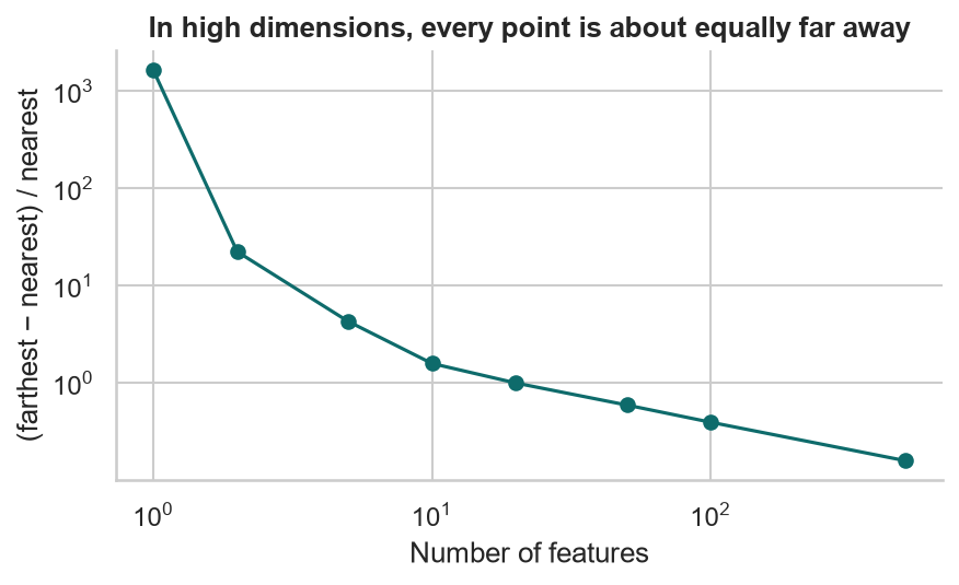
500 random points; how much farther is the farthest than the nearest?
| 2 features | 22× |
| 10 features | 1.6× |
| 100 features | 0.40× |
| 500 features | 0.16× |
When every point is about equally far from every other, “nearest centroid” loses meaning. Keep clustering features few and purposeful, or reduce dimension first (e.g. principal components).
Choosing kElbow and silhouette
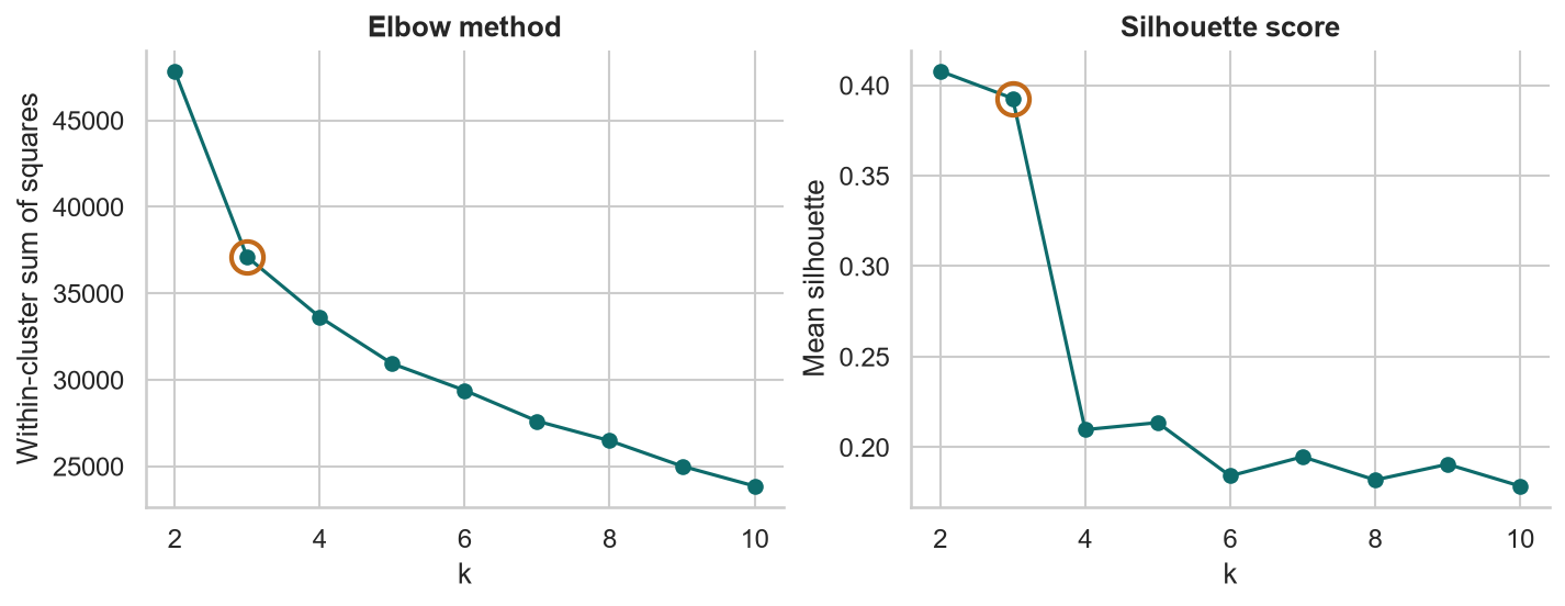
Elbow: inertia 47,844 → 37,097 → 33,628 for k = 2, 3, 4. The big gain stops after 3.
Silhouette (−1 to 1): how much closer each member is to its own cluster than to the next. 0.408 at k = 2, 0.393 at k = 3, then ≈ 0.21.
The silhouette slightly prefers 2; the elbow and the business prefer 3. Splitting off the 8% of members who drive 60% of cost is worth it. Metrics guide k; they don’t choose it.
Translating Clusters
From centroids to archetypes a care manager recognizes.
HeatmapCentroids as z-scores
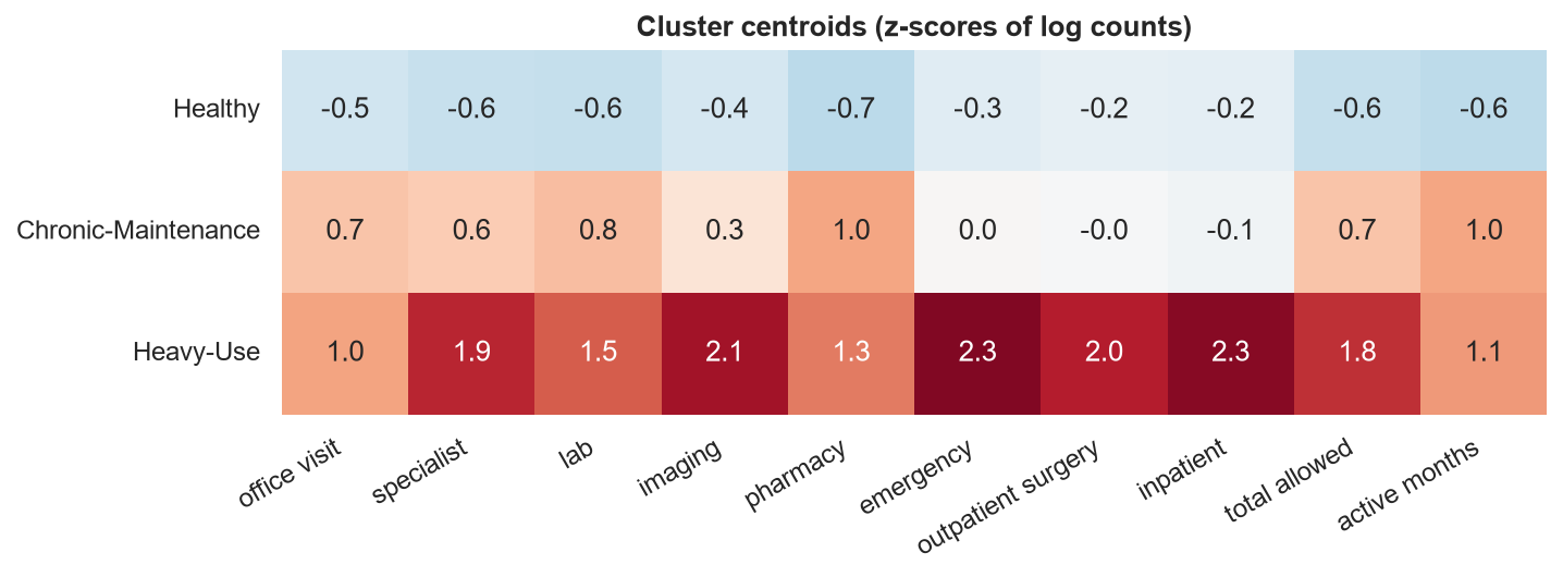
Healthy: below average on everything; active only 4 months a year.
Chronic-Maintenance: steady pharmacy and lab, 11 active months, but no more ER or inpatient use than average.
Heavy-Use: +2 sd on emergency, inpatient, imaging, and surgery.
ProfilesRadar chart and the numbers behind it
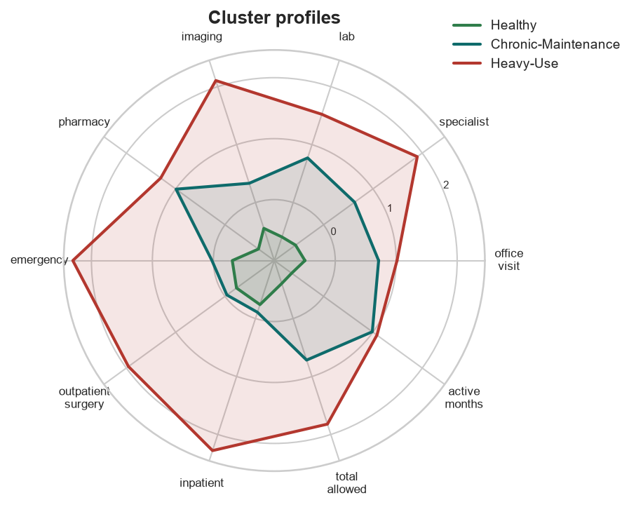
| Mean per member | Healthy | Chronic | Heavy |
|---|---|---|---|
| Members | 4,868 | 2,501 | 631 |
| Pharmacy fills | 2.4 | 26.2 | 38.6 |
| Specialist visits | 0.3 | 2.8 | 9.1 |
| Emergency visits | 0.09 | 0.33 | 2.98 |
| Inpatient stays | 0.01 | 0.05 | 1.04 |
| Active months | 4.3 | 11.3 | 11.9 |
| Allowed, 2024 | 1,419 | 9,892 | 76,017 |
| Share of members | 61% | 31% | 8% |
| Share of cost | 9% | 31% | 60% |
ValidationAre the clusters real and useful?
Against the hidden archetypes (answer key)
| True ↓ / cluster → | Healthy | Chronic | Heavy |
|---|---|---|---|
| Healthy | 4,833 | 73 | 0 |
| Chronic-Maintenance | 35 | 2,319 | 28 |
| Heavy-Use | 0 | 109 | 603 |
96.9% of members sit on the diagonal; ARI 0.926. The errors sit at the borders: heavy users having a quiet year look chronic.
Against next year’s cost (real-world test)
| Cluster (2024) | Mean 2024 | Mean 2025 | Median 2025 |
|---|---|---|---|
| Healthy | 1,419 | 3,812 | 875 |
| Chronic | 9,892 | 15,894 | 7,787 |
| Heavy-Use | 76,017 | 47,062 | 25,333 |
The groups still separate cost a year later, but they drift toward the middle: regression to the mean. Some heavy users recover; some healthy members get sick. Never price next year off this year’s extremes.
Actuarial Lab · 75 minDiscovering patient archetypes
- Build the 2024 member profile: eight category counts, total allowed, active months
- log1p-transform and standardize
- Run K-means for k = 2…10; plot inertia and silhouette
- Fit k = 3; name the clusters from their profiles
- Draw the z-score heatmap and radar chart
- Tabulate members, cost, and cost share by cluster
- Check against
archetypes.csv(ARI) and against 2025 cost - Repeat without the log, and without scaling: what changes?
Answer key
| Inertia k = 3 | 37,097 |
| Silhouette k = 2 · 3 | 0.408 · 0.393 |
| Cluster sizes | 4,868 · 2,501 · 631 |
| Heavy-Use share of cost | 60% |
| ARI vs archetypes | 0.926 |
Save the labels: Lesson 6 turns them into rules.
RecapLesson 5 checklist
- I know what clustering can and can’t tell me
- I aggregate encounters into one profile per member, keeping the zeros
- I log-transform skewed counts and standardize before K-means
- I understand why distances fail in high dimensions
- I choose k with the elbow, silhouette, and business sense
- I name clusters by their profiles
- I explain clusters with heatmaps, radar charts, and cost shares
- I validate clusters against future outcomes
Rule Extraction & Interpretability of Unsupervised Models
Centroids don’t fit in an underwriting manual. Surrogate decision trees turn clusters into a handful of readable rules.