Overfitting, Generalization & Regression Regularization
Why a model that fits the past perfectly predicts the future badly, how to measure it honestly, and how shrinkage fixes it.
Lesson 4 · OverviewBy the end of this lesson you can…
- Explain the bias–variance trade-off and recognize over- and underfitting
- Split data into training, validation, and test sets, and run K-fold cross-validation
- Describe Lasso (L1), Ridge (L2), and ElasticNet penalties and their geometry
- Standardize features correctly, inside a pipeline
- Choose the penalty strength with
LassoCV,RidgeCV, andElasticNetCV - Judge when regularization matters, and when it doesn’t
Companion notebook: lesson-04-regularization.ipynb — worked examples and self-checking exercises.
The Bias–Variance Trade-off
Too simple, too flexible, and just right.
OverfittingThirty drivers, three polynomials
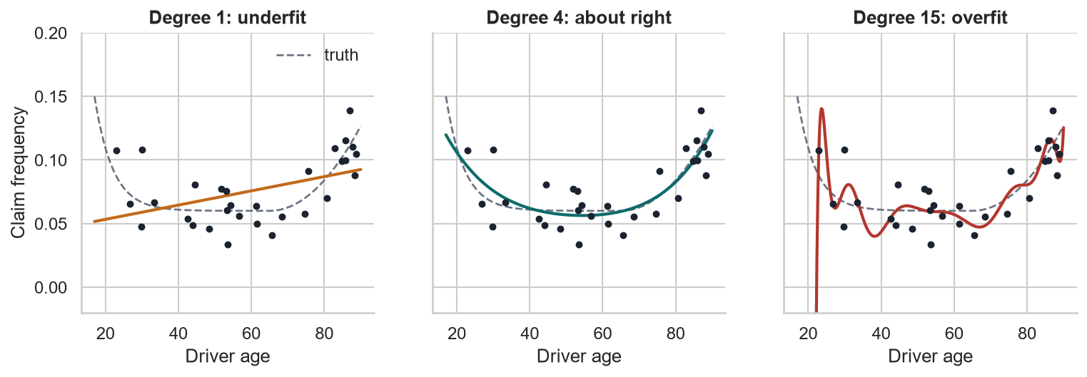
Underfit (degree 1): misses the U entirely. High bias: wrong on average, whatever sample you draw.
About right (degree 4): follows the curve, ignores the noise.
Overfit (degree 15): threads every point. High variance: a new sample gives a wildly different curve.
DecompositionExpected test error = bias² + variance + noise
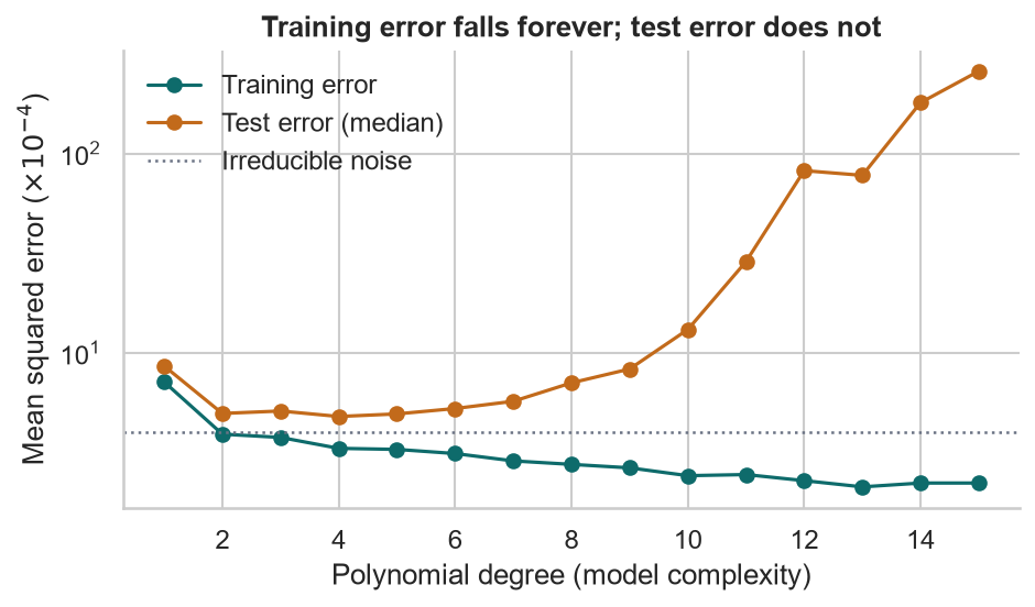
| Degree | Bias² | Variance | Test MSE |
|---|---|---|---|
| 1 | 4.03 | 0.74 | 8.58 |
| 4 | 0.10 | 1.03 | 4.79 |
| 10 | 0.94 | 110 | 13.1 |
| 15 | 5.91 | 409 | 259 |
×10⁻⁴; averaged over 200 training samples of 30 drivers. The noise floor is 4.0.
Training error always falls as complexity rises. It can’t tell you when to stop. Only data the model hasn’t seen can.
ValidationHonest measurement
Train / validation / test
from sklearn.model_selection import train_test_split
X_tr, X_te, y_tr, y_te = train_test_split(
    X, y, train_size=500, random_state=42)
Every time you look at the test score and change something, the test set becomes a validation set. Its score stops being honest.
K-fold cross-validation
Split the training data into K folds; fit on K − 1, score on the one left out; rotate; average. Every row is validated exactly once.
from sklearn.model_selection import KFold, cross_val_score
kf = KFold(5, shuffle=True, random_state=0)
cross_val_score(ols_pipe, X_tr, y_tr, cv=kf, scoring="r2")
# [0.240 0.232 0.319 0.384 0.370]  mean 0.309
Insurance rows aren’t independent: one policyholder renews for years. Use GroupKFold on the policyholder so the same person never sits on both sides of a split. For pricing, also hold out a whole later year.
A High-Dimensional Cost Model
60 features, many correlated, some pure noise.
The dataPredict next year’s cost from this year’s member
bio = pd.read_csv("data/health/biometrics.csv")
# member demographics + 8 chronic conditions
# + 2024 wellness screening (BMI, blood pressure, labs…)
# + 20 lifestyle survey items
# + 2024 encounter counts by category + log 2024 cost
X = pd.get_dummies(features, columns=["sex", "plan", "region"],
                   drop_first=True, dtype=float)
y = np.log1p(cost_2025)        # mean 7.75, sd 1.84
X.shape                        # (8000, 60)
To mimic a small employer group, we fit on 500 members and test on the other 7,500.
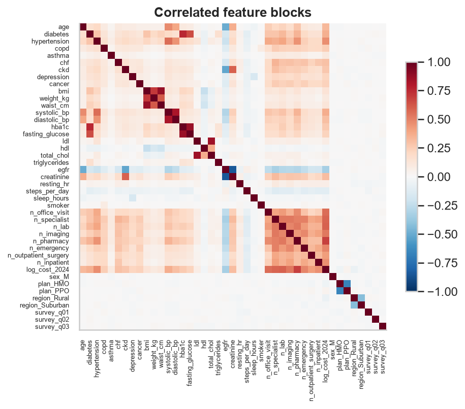
Seven pairs have |r| > 0.7: BMI–waist 0.87, HbA1c–glucose 0.87, LDL–total cholesterol 0.85, eGFR–creatinine −0.85…
OLSSixty coefficients from 500 members
from sklearn.pipeline import make_pipeline
from sklearn.preprocessing import StandardScaler
from sklearn.linear_model import LinearRegression

ols = make_pipeline(StandardScaler(), LinearRegression())
ols.fit(X_tr, y_tr)
r2_score(y_tr, ols.predict(X_tr))   # 0.482
r2_score(y_te, ols.predict(X_te)) # 0.292- Training R² 0.48; test R² 0.29: a large generalization gap
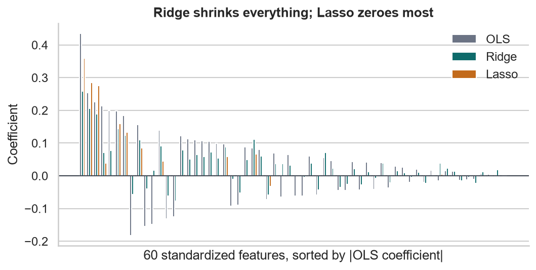
- The 20 survey items have no effect on cost, yet OLS gives them coefficients summing to 0.90 in absolute value
- Correlated blocks get large, offsetting coefficients: weight +0.200, waist −0.183
With few observations per parameter, OLS fits the noise. Its estimates are unbiased but have enormous variance, and correlated features make it worse: (X⊤X)−1 blows up when columns are nearly collinear.
Regularization accepts a little bias in exchange for a large cut in variance, by penalizing large coefficients.
Shrinkage Methods
Lasso, Ridge, and ElasticNet.
PenaltiesThree loss functions
$$\textbf{Ridge:}\;\; \min_\beta\; \tfrac{1}{2n}\lVert y - \mathbf{X}\beta\rVert^2 + \alpha\lVert\beta\rVert_2^2$$
$$\textbf{Lasso:}\;\; \min_\beta\; \tfrac{1}{2n}\lVert y - \mathbf{X}\beta\rVert^2 + \alpha\lVert\beta\rVert_1$$
$$\textbf{ElasticNet:}\;\; \ldots + \alpha\big(\rho\lVert\beta\rVert_1 + \tfrac{1-\rho}{2}\lVert\beta\rVert_2^2\big)$$
α sets the strength; ρ (l1_ratio) the mix. The intercept is never penalized.
| Ridge (L2) | Lasso (L1) | ElasticNet | |
|---|---|---|---|
| Shrinks coefficients | Smoothly toward 0 | Toward 0, many to exactly 0 | Both |
| Feature selection | No | Yes | Yes |
| Correlated group | Shares the weight | Picks one, often arbitrarily | Keeps the group together |
| Best when | Many small effects, multicollinearity | A few real effects among many | Correlated blocks + sparsity |
GeometryWhy the Lasso produces zeros
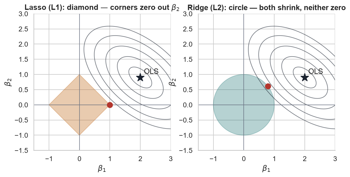
Penalized fitting is the same as minimizing the RSS inside a budget region.
- The L1 diamond has corners on the axes. The RSS ellipses usually touch it first at a corner, where some coefficients are exactly zero
- The L2 circle has no corners: coefficients shrink but stay non-zero
Tighter budget (larger α) → smaller region → more shrinkage.
ScalingStandardize first — inside the pipeline
The penalty treats every coefficient alike, but a coefficient’s size depends on its feature’s units. Steps per day (sd 3,529) needs a tiny coefficient; diabetes (sd 0.36) a large one. Without scaling, the penalty barely touches the first and crushes the second.
# ✅ scaler learns mean/sd from each training fold only
lasso = make_pipeline(StandardScaler(), LassoCV(cv=kf))

# ❌ unscaled: same α, different model
Lasso(alpha=0.107).fit(X_tr, y_tr)
# keeps 20 features incl. steps_per_day and two survey items
# test R² 0.322 (scaled: 0.355)
Leakage pitfall: StandardScaler().fit(X) on all rows before splitting lets test-set means into training. Put the scaler in a Pipeline so cross-validation refits it on every fold.
Coefficients are now “per standard deviation”. To report them in original units, divide by the scaler’s scale_.
Scale 0/1 dummies too? It’s a choice: after scaling, rare levels are penalized less. Be consistent, and say which you did.
Tuning αCross-validation picks the penalty
from sklearn.linear_model import LassoCV, RidgeCV, ElasticNetCV

lasso = make_pipeline(StandardScaler(),
                      LassoCV(cv=kf, random_state=0)).fit(X_tr, y_tr)
lasso[-1].alpha_               # 0.107
(lasso[-1].coef_ != 0).sum()   # 13 of 60

ridge = make_pipeline(StandardScaler(),
          RidgeCV(alphas=np.logspace(-2, 4, 60), cv=kf))
enet = make_pipeline(StandardScaler(),
          ElasticNetCV(l1_ratio=[0.1, 0.5, 0.9], cv=kf))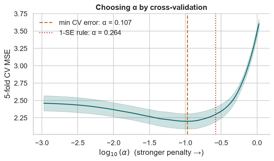
The 1-SE rule picks the largest α within one standard error of the minimum: a simpler model (7 features, test R² 0.329) that’s statistically as good.
ResultsTest-set scoreboard (7,500 members)
| Model | α | Train R² | Test R² | Test RMSE | Features |
|---|---|---|---|---|---|
| OLS | — | 0.482 | 0.292 | 1.548 | 60 |
| Ridge | 298 | 0.458 | 0.341 | 1.494 | 60 |
| Lasso | 0.107 | 0.424 | 0.355 | 1.477 | 13 |
| ElasticNet (ρ = 0.5) | 0.199 | 0.425 | 0.357 | 1.476 | 16 |
Every penalized model has a lower training R² and a higher test R² than OLS. That’s the trade-off working.
SelectionWhat the Lasso kept
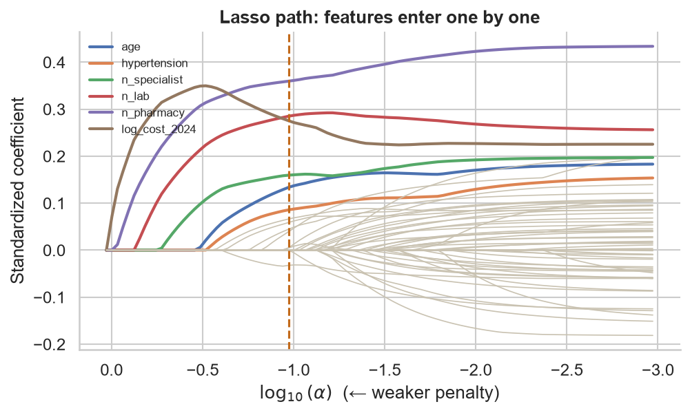
Prior utilization enters first and beats every biometric.
Survey item q04 (β = 0.005) is noise that slipped through; the 1-SE model drops it.
| Feature (standardized) | Lasso | OLS |
|---|---|---|
| n_pharmacy | 0.360 | 0.435 |
| n_lab | 0.285 | 0.254 |
| log_cost_2024 | 0.275 | 0.226 |
| n_specialist | 0.160 | 0.197 |
| hypertension · diabetes | 0.086 · 0.045 | 0.157 · 0.139 |
| bmi · weight · waist | 0 · 0 · 0 | −0.020 · 0.200 · −0.183 |
| 20 survey items (sum of |β|) | 0.005 | 0.899 |
PerspectiveWhen does regularization matter?
| Training members | OLS test R² | Lasso test R² |
|---|---|---|
| 200 | 0.115 | 0.331 |
| 500 | 0.292 | 0.355 |
| 1,000 | 0.334 | 0.355 |
| 2,000 | 0.353 | 0.353 |
| 4,000 | 0.352 | 0.354 |
| 7,000 | 0.347 | 0.350 |
With enough data per feature, OLS catches up. Regularization matters most when data is thin relative to the number of parameters:
- Small employer groups, new products, rare coverages
- Many-level factors: vehicle model, ZIP code, diagnosis code
- Interactions: 6 styles × 8 ages × 100 counties is 4,800 cells
Penalized GLMs are credibility in modern dress: thin cells shrink toward the overall mean, just as Bühlmann credibility shrinks toward the collective. Lesson 8 uses a penalized Poisson GLM.
Actuarial Lab · 75 minRegularizing a 60-feature claim cost model
- Build the member feature table: members, biometrics, 2024 encounter counts, log 2024 cost
- Target: log(1 + 2025 cost). Split 500 train / 7,500 test with
random_state=42 - Fit OLS in a pipeline; record train and test R²
- Fit
RidgeCV,LassoCV,ElasticNetCVwith 5-fold CV - Which features survive the Lasso? What happened to the survey items and to BMI / weight / waist?
- Apply the 1-SE rule; refit; compare
- Repeat the OLS vs Lasso comparison at 200 and 2,000 training members
Answer key
| OLS test R² | 0.292 |
| RidgeCV α · test R² | 298 · 0.341 |
| LassoCV α · test R² | 0.107 · 0.355 |
| Lasso non-zero features | 13 |
| 1-SE α · features · test R² | 0.264 · 7 · 0.329 |
RecapLesson 4 checklist
- I can explain bias, variance, and why training error misleads
- I keep a test set untouched and tune with cross-validation
- I group folds by policyholder and hold out later years
- I know what the L1 and L2 penalties do, and why the Lasso zeroes coefficients
- I standardize inside a
Pipeline, never before the split - I tune α with
LassoCV,RidgeCV,ElasticNetCV - I know when the 1-SE rule is worth it
- I know regularization pays most when data is thin
Unsupervised Learning & Risk Group Discovery
No target, no labels: K-means finds patient archetypes hidden in 180,000 encounters.