GLMs: Severity & Pure Premium Modeling
How much claims cost, and what a policy should cost: Gamma and inverse Gaussian severity, the two-part pure premium, and the Tweedie.
Lesson 3 · OverviewBy the end of this lesson you can…
- Fit Gamma and inverse Gaussian GLMs with a log link to claim severity
- Compare severity families with residuals and likelihood
- Combine frequency and severity into a pure premium: E[loss] = E[N] × E[X]
- Turn two GLMs into a multiplicative rating algorithm
- Fit a Tweedie GLM to pure premium in one step and choose its power
- Check a model on the holdout year with actual ÷ expected
Companion notebook: lesson-03-severity-pure-premium.ipynb — worked examples and self-checking exercises.
Severity Models
Continuous, strictly positive, right-skewed.
The dataOne row per liability claim
claims = pd.read_csv("data/motor/claims.csv")
claims["incurred"] = claims["paid"] + claims["outstanding"]
liab = claims[claims["coverage"] == "LIAB"].merge(
    train[["vehicle_id", "vehicle_style", "age_band",
           "urban", "log_miles", "channel", "driver_age"]],
    on="vehicle_id", how="inner", validate="many_to_one")
liab["young"] = liab["driver_age"] < 25
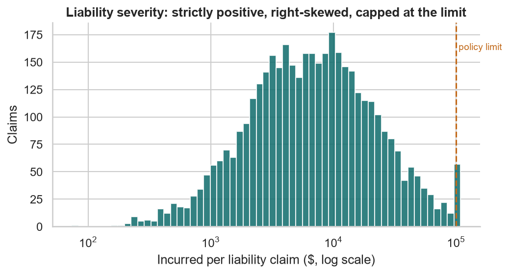
len(liab) # 4,041 claims from policy years 2021–2024| Mean · median incurred | 12,817 · 6,647 |
| Coefficient of variation | 1.36 |
| Claims at or above the 100,000 limit | 51 |
Gamma GLMConstant coefficient of variation
$$Y \sim \text{Gamma}(\mu, \phi) \qquad \mathrm{Var}(Y) = \phi\,\mu^2 \qquad \ln\mu = \mathbf{x}^\top\beta$$
gamma_log = sm.families.Gamma(sm.families.links.Log())
sev = smf.glm("incurred ~ C(vehicle_style, Treatment('Sedan'))"
              " + young + urban", data=liab,
              family=gamma_log).fit()

np.exp(sev.params)
sev.scale # dispersion 1.832 → CV = √φ = 1.35- Standard deviation ∝ mean: a $10,000 claim has 10× the spread of a $1,000 claim
- Specify the log link explicitly: the Gamma’s default is the inverse link
| Term | Relativity | 95% CI | Truth |
|---|---|---|---|
| Base (Sedan, 25+, non-urban) | 11,253 | 10,156–12,468 | — |
| Sports | 1.204 | 1.035–1.400 | 1.30 |
| Young driver (< 25) | 1.202 | 1.085–1.331 | 1.15 |
| Urban | 1.107 | 1.014–1.210 | 1.10 |
| Hatchback | 0.928 | 0.814–1.057 | 1.00 |
| SUV | 1.017 | 0.909–1.139 | 1.00 |
Severity is noisy: intervals are ±15% wide. Adding age bands, mileage, and channel adds nothing (F = 1.20, p = 0.29).
Family choiceGamma, inverse Gaussian, or lognormal?
| Family | V(μ) | AIC | Sports · young · urban |
|---|---|---|---|
| Gamma | μ² | 85,001.1 | 1.204 · 1.202 · 1.107 |
| Inverse Gaussian | μ³ | 84,687.6 | 1.203 · 1.200 · 1.109 |
| Lognormal (log-OLS) | — | 83,865.0 | 1.253 · 1.279 · 1.128 |
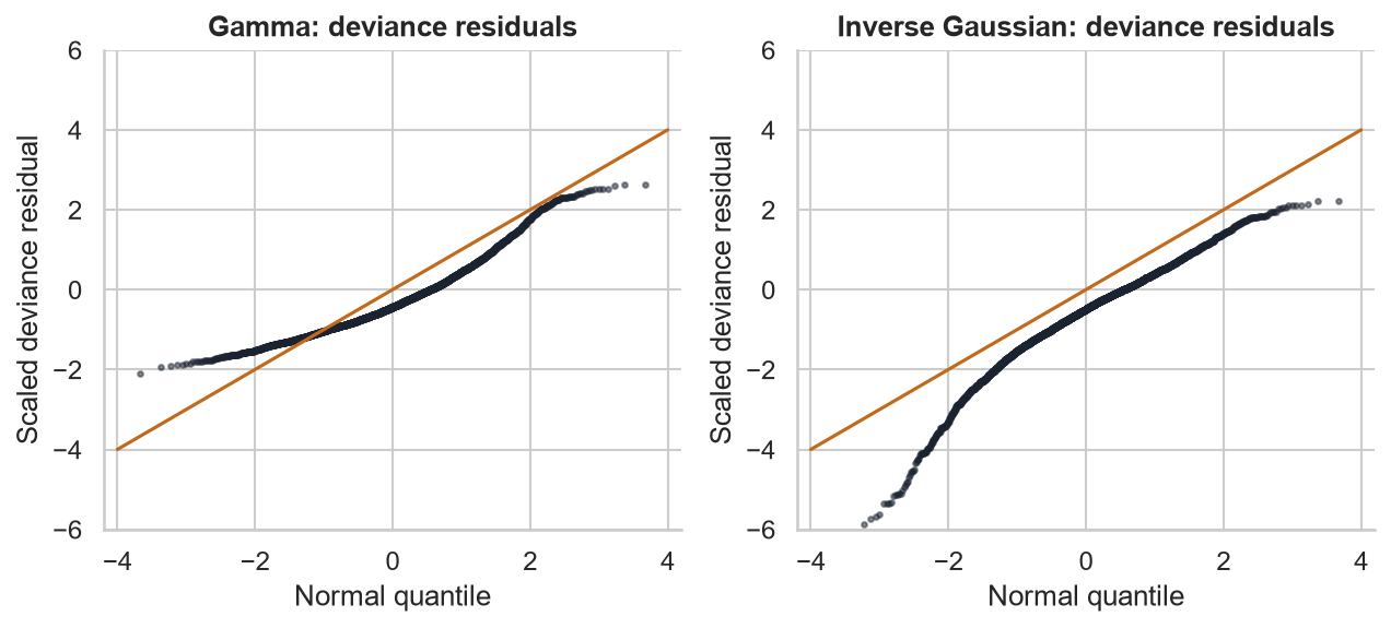
The claims were simulated lognormal, and the likelihood finds it; Gamma residuals bend away at both ends.
The relativities barely change between families. Gamma stays the default: its mean is right in dollars, and it pairs naturally with a Poisson frequency model.
The Two-Part Pure Premium
How often × how much.
Frequency × severityCombining two GLMs
$$\text{Pure Premium} = \widehat{\text{Frequency}} \times \widehat{\text{Severity}}$$
Valid when claim count and claim size are independent given the features, the standard collective-risk assumption.
# predicted rate per car-year: offset of zero = one year
train["freq_hat"] = freq.predict(train, offset=np.zeros(len(train)))
train["sev_hat"] = sev.predict(train)
train["pp_hat"] = train["freq_hat"] * train["sev_hat"]

(train["pp_hat"] * train["exposure"]).sum()   # 51,773,072
train["inc_liab"].sum()                       # 51,794,591
Because both use a log link, the pure premium is still multiplicative. Each factor’s pure-premium relativity is its frequency relativity × its severity relativity.
| Style | Freq. | Sev. | Pure prem. |
|---|---|---|---|
| Sedan (base) | 1.000 | 1.000 | 1.000 |
| Minivan | 0.856 | 0.896 | 0.767 |
| Pickup | 1.005 | 1.050 | 1.055 |
| Hatchback | 1.213 | 0.928 | 1.125 |
| SUV | 1.224 | 1.017 | 1.246 |
| Sports | 1.728 | 1.204 | 2.080 |
Rating algorithmFrom two GLMs to a rating manual
$$\text{PP} = \underbrace{447.03}_{\text{base}} \times f_{\text{style}} \times f_{\text{age}} \times f_{\text{young}} \times f_{\text{urban}} \times \Big(\tfrac{\text{miles}}{12{,}000}\Big)^{0.488}$$
| Factor | From | Values |
|---|---|---|
| Base 447.03 | 0.03973 × 11,253 | Sedan, 40–49, non-urban, 12,000 mi |
| Age band | frequency | 17–20: 2.062 · 21–24: 1.767 · 25–29: 1.279 · 75+: 1.680 |
| Young driver | severity | under 25: 1.202 |
| Urban | both | 1.365 × 1.107 = 1.512 |
| Mileage | frequency | elasticity 0.488 |
Three risks, priced
| Risk | Freq. | Sev. | Pure prem. |
|---|---|---|---|
| Sedan · 40–49 · rural · 12k mi | 0.0397 | 11,253 | 447.03 |
| Sports · 17–20 · urban · 15k mi | 0.2154 | 18,028 | 3,883.87 |
| Minivan · 50–64 · urban · 8k mi | 0.0370 | 11,164 | 412.67 |
A premium is the pure premium plus expenses and profit: premium = PP ÷ permissible loss ratio. Lesson 8’s capstone turns these into rate indications.
ValidationDoes it hold up next year?
for d in (train, hold):
    d["pp_hat"] = (freq.predict(d, offset=np.zeros(len(d)))
                   * sev.predict(d))

expected = (hold["pp_hat"] * hold["exposure"]).sum()
hold["inc_liab"].sum() / expected       # A/E = 1.022
On policy year 2025, which the models never saw, actual losses were 2.2% above expected: 7,261,043 against 7,107,968.
| Training years | Non-urban | Urban |
|---|---|---|
| Liability premium per car-year | 1,104 | 1,096 |
| Actual pure premium | 627 | 937 |
| Model pure premium | 628 | 935 |
| Loss ratio | 56.8% | 85.4% |
The current rating plan charges urban and rural drivers the same, yet urban cars cost 50% more. The model sees it; the rates don’t. That gap is what a pricing review exists to close.
The Tweedie Model
Pure premium in a single GLM.
Compound Poisson–GammaA distribution with a mass at zero
$$S = \sum_{j=1}^{N} X_j,\quad N \sim \text{Poisson},\; X_j \sim \text{Gamma}$$
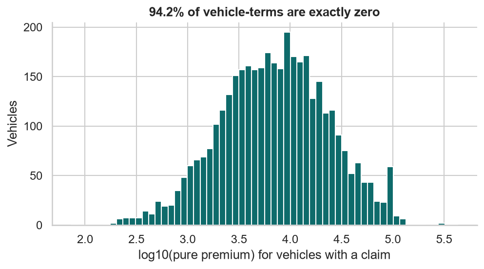
S is exactly zero when N = 0, and continuous otherwise. It belongs to the EDF with
$$\mathrm{Var}(S) = \phi\,\mu^p, \qquad 1 < p < 2$$
- p → 1: Poisson-like (counts)
- p → 2: Gamma-like (sizes)
- Model pure premium directly, with exposure as a weight
statsmodelsFitting a Tweedie GLM
train["pp"] = train["inc_liab"] / train["exposure"]

tw = smf.glm("pp ~ C(vehicle_style, Treatment('Sedan'))"
             " + C(age_band, Treatment('40-49'))"
             " + urban + log_miles",
             data=train, var_weights=train["exposure"],
             family=sm.families.Tweedie(
                 var_power=1.6, link=sm.families.links.Log()),
).fit()| Power p | 1.3 | 1.4 | 1.5 | 1.6 | 1.7 | 1.8 |
|---|---|---|---|---|---|---|
| Log-lik. (000s) | −58.7 | −56.2 | −55.0 | −54.7 | −54.9 | −56.3 |
Choose p by profile likelihood: fit a grid, keep the best.
| Relativity | Tweedie | Freq × sev |
|---|---|---|
| Base | 431.53 | 447.03 |
| Sports | 1.961 | 2.080 |
| Age 17–20 | 2.600 | 2.062 × 1.202 = 2.477 |
| Age 21–24 | 2.253 | 1.767 × 1.202 = 2.124 |
| Urban | 1.516 | 1.512 |
| log_miles β | 0.447 | 0.488 |
Holdout A/E: Tweedie 1.025, two-part 1.022.
Trade-offsTwo-part or Tweedie?
Frequency × severity
- Shows why a segment is expensive: more claims, or bigger ones?
- Different features in each part (age drives frequency, not severity)
- Two models to fit, validate, and maintain
- Needs claim-level data
Tweedie
- One model, one set of relativities
- Works on policy-level aggregate losses: no claim file needed
- Assumes every factor moves frequency and severity together
- The popular loss for gradient boosting (Lesson 7)
Many pricing teams build both: the two-part model for insight and filing support, the Tweedie as a cross-check. When they disagree, find out why.
Actuarial Lab · 75 minA prospective policy rating algorithm
- Build the claim-level severity table for policy years ≤ 2024
- Fit a Gamma log-link GLM; F-test the full against the parsimonious model
- Refit with inverse Gaussian; compare relativities and AIC
- Refit Lesson 2’s reduced Poisson model; predict frequency, severity, pure premium
- Write
rate(style, age_band, young, urban, miles)from the fitted factors - Check A/E on the 2025 holdout
- Fit a Tweedie over p = 1.3…1.8; compare with the two-part model
Answer key
| Gamma base severity | 11,253.05 |
| Gamma dispersion φ | 1.832 |
| Base pure premium | 447.03 |
| Sports · 17–20 · urban · 15k | 3,883.87 |
| Training: expected ÷ actual | 0.9996 |
| Holdout A/E (two-part) | 1.022 |
| Best Tweedie power | 1.6 |
RecapLesson 3 checklist
- I fit severity with a Gamma GLM and an explicit log link
- I compare families by residuals and likelihood, and know relativities rarely move
- I combine frequency and severity into a pure premium
- I write the result as base rate × factors
- I check expected vs actual on training and holdout data
- I fit a Tweedie with exposure weights and choose its power
- I know when to prefer two parts or one
- I found the urban pricing gap
Overfitting, Generalization & Regularization
The bias–variance trade-off, cross-validation, and Lasso, Ridge, and ElasticNet on a 60-feature health cost model.