Capstone: An End-to-End Rating Engine & Report
Operational database dumps in; exposure, loss ratios, spatial territories, and rate indications out — as an executive Excel report and a Reveal.js deck.
The briefWhat you’re building
The head of motor pricing wants a quarterly rating review that anyone on the team can reproduce with one command:
- Ingest the six-table operational dump and validate it
- Compute exact earned exposure and earned premium to the evaluation date
- Enrich every vehicle with a spatial territory
- Calculate segment experience and credibility-weighted rate indications
- Report: an executive Excel workbook and a Reveal.js slide deck
Uses every lesson
Cleaning (1) · exposure (2) · joins (3) · metrics (4) · charts (5) · spatial (6) · Excel (7) · pipelines (8A)
Why it matters
This is what a pricing team’s quarterly process looks like when it’s done well: fast, reproducible, reviewable.
Companion notebook: lesson-08b-capstone.ipynb — worked examples and self-checking exercises.
Requirements
Inputs, stages, and outputs.
SpecificationInputs and outputs
Inputs
data/motor/*.csv— the six-table schema (Lesson 3)data/geo/nc_geo.gpkg— counties, places, coastline (Lesson 6)config.toml— evaluation date, territory rule, age bands, indication parameters
Command
uv run rating-pipeline --config config.tomlOutputs (in output/)
abt.parquet | the enriched vehicle-level ABT |
rating_review.xlsx | Summary (KPI cards), Territory, Segments (territory × age band with indications, loss ratios above target highlighted) |
rating_review.html | a Reveal.js deck: title, KPIs, territory chart and table, largest proposed changes |
figures/*.png | charts used by the deck |
| run log | row counts, control totals, file paths |
CalculationThe indication, step by step
def indicate(seg, target_loss_ratio, annual_trend, trend_years,
             full_credibility_claims, max_change):
    out = seg.copy()
    out["trended_lr"] = (out["loss_ratio"]
                         * (1 + annual_trend) ** trend_years)
    out["indicated_change"] = (out["trended_lr"]
                               / target_loss_ratio - 1)
    out["credibility"] = np.minimum(
        1, np.sqrt(out["claims"] / full_credibility_claims))
    out["proposed_change"] = (out["credibility"]
                              * out["indicated_change"]
                             ).clip(-max_change, max_change)
    return out

segments = indicate(experience(abt, ["territory", "age_band"]),
**cfg["indication"])- Trend the experience loss ratio 1.5 years forward at 4% a year
- Indicate: how far above or below the 68% target is it?
- Credibility: Z = min(1, √(claims ÷ 1,082)) — thin segments move less
- Cap at ±15% so no customer sees a shock
Identical logic to the Lesson 7 Excel panel — and the two independent implementations agree: +7.8% premium-weighted proposed change.
Generating the Slide Deck
HTML from a template — the same Reveal.js you’ve watched all course.
Jinja2Templates: HTML with holes in it
<!-- templates/deck.html.j2 -->
<section>
  <h2>Portfolio at a glance</h2>
  <div class="kpi"><b>{{ "{:.1%}".format(kpis.loss_ratio) }}</b>
    loss ratio</div>
</section>
<section>
  <h2>Loss ratio by territory</h2>
  <img src="figures/territory_lr.png">
  <table>
  {% for t in territory %}
    <tr><td>{{ t.territory }}</td>
        <td class="{{ 'over' if t.loss_ratio > params.target_loss_ratio }}">
          {{ "{:.1%}".format(t.loss_ratio) }}</td></tr>
  {% endfor %}
  </table>
</section>
from jinja2 import (Environment, PackageLoader,
select_autoescape)
env = Environment(loader=PackageLoader("rating_pipeline"),
autoescape=select_autoescape())
html = env.get_template("deck.html.j2").render(
kpis=kpis,
territory=territory.to_dict("records"),
params=params)
Path("output/rating_review.html").write_text(html){{ … }}inserts a value;{% for %}/{% if %}control structure- Pass plain Python data:
to_dict("records")gives a list of row dicts autoescapestops text in the data being read as HTML
The deck is regenerated with the numbers every run — no copy-paste into PowerPoint, ever again.
ResultThe generated deck
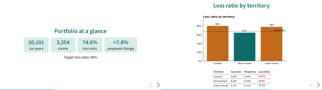
Two slides from a finished pipeline’s output/rating_review.html.
Answer keyYour pipeline should reproduce these
| Control totals | |
|---|---|
| Policy terms · vehicles | 22,185 · 23,993 |
| Car years | 20,100.95 |
| Claims · incurred | 3,354 · 24,669,862 |
| Portfolio loss ratio | 74.6% |
| Premium-weighted proposed change | +7.8% |
| Territory | Vehicles | Car years | Freq. | LR |
|---|---|---|---|---|
| Coastal | 4,834 | 4,070.0 | 0.1907 | 80.5% |
| Rural inland | 7,501 | 6,284.0 | 0.1440 | 64.9% |
| Urban inland | 11,658 | 9,746.9 | 0.1716 | 78.3% |
Largest proposals: Urban inland 35–49, Coastal 75+, Urban inland 17–24 and 25–34 at the +15% cap; Coastal 50–64 at +12.4%.
Small differences in the fourth significant figure usually mean a different exposure convention or age-band edge. Larger ones mean a join changed the grain — check your control totals.
Capstone deliverableWhat to hand in
1 · The repository
- A
uvpackage with the four stage modules and a CLI entry point config.tomlholding every assumptionREADME.md: what it does, how to run it, what it producesoutput/git-ignored;uv.lockcommitted
2 · Tests
- Exposure (leap year, cancellation, in force at evaluation)
- Metrics are ratios of sums; indication capping and credibility
- A data-quality test: a duplicated key raises
DataQualityError
3 · The outputs
rating_review.xlsxstyled to the corporate paletterating_review.htmlgenerated from a Jinja2 template, with at least one chart- A run log from a clean run
4 · A one-page memo
- Where the current rates are inadequate, and by how much
- What the territory analysis changes
- The limitations: incurred not ultimate, no IBNR, thin segments
Definition of done: a fresh clone, uv sync, uv run rating-pipeline, uv run pytest — all green, no manual steps.
AssessmentHow it will be marked
| Criterion | Weight | What “excellent” looks like |
|---|---|---|
| Correctness | 30% | Reproduces the answer key; every control total reconciles |
| Architecture | 20% | Clean stages, I/O at the edges, all parameters in config, one-command run |
| Data quality & tests | 15% | Key and grain checks that stop bad runs; meaningful, fast tests |
| Reporting | 20% | Excel and slides a pricing committee could use unedited; headline titles; formatted numbers |
| Judgment | 15% | Memo is honest about credibility and limitations; recommendations follow from the evidence |
Stretch goalsIf you finish early
Honor the evaluation date
Set date = 2024-12-31 in the config. Exclude policies incepting and claims reported after it, and cap every open claim’s development at that date. What changes?
Messy input
Point the pipeline at claims_raw.csv (Lesson 1) and add a cleaning stage with a rejects report in the Excel workbook.
A map in the deck
Add the Lesson 6 county choropleth to the generated slides, masked for credibility.
The first stretch goal is the most important in practice: a pipeline that quietly uses data from after its evaluation date produces results nobody could have known at the time — a serious error in reserving and pricing work.
Course 2 · RecapEight lessons, one pipeline
1 · pandas
Clean a messy extract; log what you drop2 · Dates
Exact exposure; CY, PY, AY3 · Joins
Keys, grain, and an ABT that reconciles4 · Metrics
Frequency, severity, pure premium, LR5 · EDA
Charts that make a point6 · Spatial
Territories from real geography7 · Excel
Live, tested workbooks by code8 · Pipelines
One command, every quarterYou can now take real, messy, multi-table data all the way to a decision-ready report.
Predictive Modeling & Modern Actuarial Machine Learning
From one-way tables to GLMs, gradient boosting, and interpretable risk models — on a larger motor book and a health-claims book, built with the skills you just practiced.