Python for Actuarial Students · Course 2

Lesson 6

Programmatic Spatial Data Analysis

GeoPackages, coordinate reference systems, and spatial joins — rating territories and coastal risk, without leaving Python.

Lesson 6 · OverviewBy the end of this lesson you can…

Read shapefiles and GeoPackages into a GeoDataFrame
Explain coordinate reference systems and choose one fit for measuring distance
Turn latitude/longitude columns into points, and reproject them
Assign policies to territories with gpd.sjoin — and handle the misses
Build geographic risk proxies: urban density and distance to the coast
Map rating results as a credibility-aware choropleth

75 min

Concepts & worked examples

75 min

Lab: territory rating factors

Companion notebook: lesson-06-spatial-analysis.ipynb — worked examples and self-checking exercises.

WhyReplacing the desktop GIS

Territory work has traditionally meant exporting a CSV, opening QGIS, clicking through a spatial join, exporting again, and re-importing into Excel.

Not repeatable — next quarter, click it all again
Not reviewable — no record of which layer or setting was used
Not connected to the pricing data pipeline

geopandas is pandas with a geometry column. Everything from Lessons 1–5 still works; spatial operations are added on top.

Our data: real North Carolina geography — 100 counties and 777 incorporated places (US Census 2023), and the coastline (Natural Earth) — with 23,993 synthetic insured vehicles.

Part 1

Geospatial Data

File formats, geometries, and the GeoDataFrame.

FormatsShapefiles and GeoPackages

	Shapefile	GeoPackage
Files	4+ (`.shp`, `.shx`, `.dbf`, `.prj`…) that must travel together	one `.gpkg`
Layers	one per file set	many in one file
Column names	max 10 characters	unlimited
Standard	1990s de facto	open OGC standard (SQLite)

Census boundaries still ship as zipped shapefiles — gpd.read_file("x.zip") reads them directly. Save your working data as GeoPackage.

import geopandas as gpd
import pyogrio

pyogrio.list_layers("data/geo/nc_geo.gpkg")
# [['counties'  'Polygon']
#  ['places'    'MultiPolygon']
#  ['coastline' 'LineString']]

counties = gpd.read_file("data/geo/nc_geo.gpkg",
                         layer="counties")
counties.head(3)
#   county_fips county_name  geometry
# 0       37095        Hyde  POLYGON ((…))
# 1       37113       Macon  POLYGON ((…))
# 2       37069    Franklin  POLYGON ((…))

GeoDataFrameA DataFrame with a geometry column

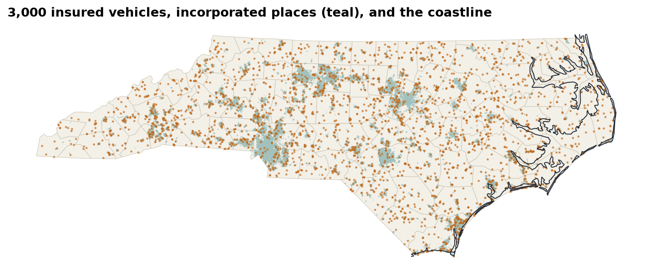
Map of North Carolina counties with incorporated places shaded teal, the coastline in dark ink, and 3,000 insured vehicles as small amber dots concentrated around Charlotte, the Triangle, and the Triad

Points

Vehicles’ garaging locations

Lines

The coastline — 12 pieces

Polygons

Counties; places (multi-part)

Each layer draws with .plot(ax=ax) — stack them on one axes to build a map.

Part 2

Coordinate Reference Systems

Numbers only mean a place once you say which system they’re in.

CRSDegrees, meters, and EPSG codes

EPSG	Name	Units	Use for
`4326`	WGS 84	degrees	storing lat/long, GPS
`3857`	Web Mercator	“meters”	web map tiles only
`32119`	NAD83 / North Carolina	meters	distances & areas in NC

counties.crs          # EPSG:32119
pts.to_crs(counties.crs)          # reproject (pyproj)
pts.set_crs("EPSG:4326")          # LABEL only — no math

Raleigh → Wilmington, measured four ways:

In EPSG:4326 (degrees)	1.7016 “units”
In EPSG:3857 (Web Mercator)	224.86 km
In EPSG:32119 (state plane)	183.63 km
Geodesic on the ellipsoid (`pyproj.Geod`)	183.65 km

Web Mercator stretches distances by 1/cos(latitude) — here 22% too long. Measure in a local projected CRS, never in degrees or Web Mercator.

PointsFrom latitude/longitude columns to geometry

abt = pd.read_parquet("data/processed/abt.parquet")

pts = gpd.GeoDataFrame(
    abt,
    geometry=gpd.points_from_xy(abt["longitude"],   # x first!
                                abt["latitude"]),   # then y
    crs="EPSG:4326",                  # what the numbers ARE
).to_crs("EPSG:32119")                # what we want to measure in

points_from_xy(x, y): longitude is x, latitude is y. Swap them and North Carolina lands in Antarctica
crs= declares the system the raw numbers are in
.to_crs() transforms coordinates; .set_crs() only relabels
Bring every layer into the same CRS before combining them

Sanity check: pts.total_bounds should sit inside counties.total_bounds. Plot them together — a misplaced CRS is obvious on a map.

Part 3

Spatial Joins

Merging on where instead of on a key.

sjoinWhich county is each vehicle in?

j = gpd.sjoin(pts,
              counties[["county_fips", "county_name", "geometry"]],
              how="left", predicate="within")

len(j)                          # 23993 — no duplicates
j["county_fips"].isna().sum()   # 12 — unmatched!
j = j.drop(columns="index_right")

Why 12 misses? The county file is generalized (the 1:20m version) — smoothed coastlines cut off a few waterfront addresses. gpd.sjoin_nearest(misses, counties, max_distance=2_000) assigns all 12; the furthest is 767 m away.

`predicate=`	Keeps pairs where the left geometry…
`within`	lies inside the right
`intersects`	touches or overlaps it
`contains`	encloses it

Same discipline as Lesson 3: check the row count (a point in two overlapping polygons appears twice) and the unmatched count. sjoin_nearest with a max_distance rescues near-misses without inventing far-away matches.

Urban densityInside a town or not?

places = gpd.read_file("data/geo/nc_geo.gpkg", layer="places")

u = gpd.sjoin(j[["vehicle_id", "geometry"]],
              places[["place_name", "geometry"]],
              how="left", predicate="within")
u["vehicle_id"].duplicated().sum()     # 0
j["urban"] = u.set_index("vehicle_id") \
              .loc[j["vehicle_id"], "place_name"].notna().to_numpy()

j["urban"].mean()                      # 0.5943

	Rural	Urban	Ratio
COLL frequency	0.0769	0.0953	1.24×
COLL loss ratio	84.7%	103.1%
LIAB frequency	0.0552	0.0713	1.29×
LIAB loss ratio	59.0%	71.6%

More traffic, more collisions. The rating plan charges town and country alike, so urban risks run ~20 loss-ratio points worse. Incorporated place boundaries are a crude density proxy; census urban-area or population-density layers are better.

Part 4

Geographic Risk Proxies

Distances, buffers, and territory schemes.

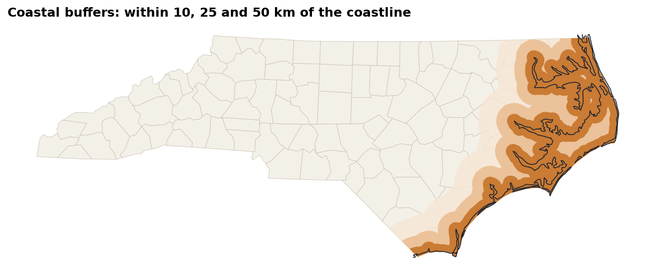
ProximityDistance to the coastline

coast = gpd.read_file("data/geo/nc_geo.gpkg", layer="coastline")
coastline = coast.union_all()        # one geometry

j["coast_km"] = j.geometry.distance(coastline) / 1000
j["coast_band"] = pd.cut(j["coast_km"],
    [0, 10, 25, 50, 100, 1000], right=False,
    labels=["<10 km", "10–25", "25–50", "50–100", "100+"])

Band	COMP exposure	COMP freq.	COMP LR
<10 km	2,431	0.0650	194.8%
10–25	964	0.0633	188.3%
25–50	1,027	0.0506	202.7%
50–100	1,720	0.0250	87.6%
100+	10,844	0.0276	85.0%

Map of North Carolina with buffers shaded at 10, 25 and 50 kilometres from the coastline, covering the eastern third of the state around the sounds

MappingA credibility-aware choropleth

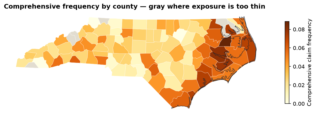
County choropleth of comprehensive claim frequency: dark orange to brown along the coast and sounds, pale yellow across the Piedmont, a few mountain counties moderately elevated, and thin-exposure counties shaded gray

m = counties.merge(county_comp, on="county_fips", validate="one_to_one")
m.loc[m["exposure"] < 60, "frequency"] = np.nan    # too thin to show
m.plot(column="frequency", cmap="YlOrBr", legend=True,
       missing_kwds={"color": "#e2ddd0"})

Lesson 4’s puzzle solved: the Mountains’ high comprehensive loss ratio isn’t coastal — all 3,768 mountain car years are 100+ km from the sea. It’s a handful of noisy mountain counties. The coastal effect, by contrast, is consistent and large.

TerritoriesFrom proxies to a rating territory

j["territory"] = np.select(
    [j["coast_km"] < 25, j["urban"]],
    ["Coastal", "Urban inland"],
    default="Rural inland")

portfolio_pp = j["incurred"].sum() / j["exposure"].sum()
t = j.groupby("territory").agg(
        exposure=("exposure", "sum"), claims=("n_claims", "sum"),
        incurred=("incurred", "sum"), premium=("earned_premium", "sum"))
t["pure_premium"] = t["incurred"] / t["exposure"]
t["relativity"] = t["pure_premium"] / portfolio_pp
t["loss_ratio"] = t["incurred"] / t["premium"]

Territory	Exposure	Freq.	Pure prem.	Relativity	LR
Coastal	4,070	0.1907	1,317	1.073	80.5%
Urban inland	9,747	0.1716	1,293	1.053	78.3%
Rural inland	6,284	0.1440	1,067	0.870	64.9%

np.select takes the first true condition — so a town on the coast counts as Coastal. Order the conditions by priority, and document it.

The flat 1.15 territory load in today’s rates overcharges rural drivers and undercharges everyone else.

Actuarial Lab · 75 minTerritory rating factors, in code

Read the three layers; confirm they share EPSG:32119
Build vehicle points from the ABT; reproject
sjoin to counties; rescue the 12 misses with sjoin_nearest
sjoin to places → urban flag (59.4%)
Distance to coast → coast_km and coast_band
Coverage-level metrics by urban and by coast_band
Three-territory scheme with relativities
Save the enriched ABT as a GeoPackage layer and a Parquet file

Answer key

Vehicles	23,993
Unmatched after `within`	12
Urban share	59.43%
Median distance to coast	164.9 km
COMP freq. <10 km vs. 100+	0.0650 vs. 0.0276
Coastal relativity	1.073

The same pattern works for any boundary layer: US Census tracts or ZIP code tabulation areas (TIGER/Line), UK postcode sectors or LSOAs (ONS Open Geography). Only the file changes.

RecapLesson 6 checklist

I can read shapefiles and GeoPackages, and list a GeoPackage’s layers
I know EPSG:4326 from a projected CRS, and to_crs from set_crs
I build points with longitude as x
I measure distances only in a projected CRS

I check row and unmatched counts after every sjoin
I built urban and coastal risk proxies
I mask thin cells on a choropleth
I derived territory relativities: 1.073 / 1.053 / 0.870

Up next

Lesson 7

Automated Excel Engineering with openpyxl

Styled, formula-driven workbooks built by code — including an interactive underwriting panel.

← Course home Next: Lesson 7 →